A novel methodology for identification of inhomogeneities in

A novel methodology for identification of inhomogeneities in climate time series Andrés Farall 1, Jean-Phillipe Boulanger 1, Liliana Orellana 2 1 CLARIS LPB Project - University of Buenos Aires 2 Biostatistics Unit - Deakin University CLARIS LPB. A Europe-South America Network for Climate Change Assessment and Impact Studies in La Plata Basin 1

Climate time series. Quality control Climatology relies on observational data to understand the climate In order to accurately monitor long-term marine or atmospheric climate change the quality of the data is of utmost importance One key challenge is to discriminate the climatic signal from noise generated by errors or inhomogeneities Errors and inhomogeneities are due to changes in the conditions data are measured, recorded, transmitted and/or stored

Quality control Instant change ⇒ Error Detection of atypical data Lasting change ⇒ Inhomogeneity Detection of breakpoints In this talk • we will focus in the problem of detection of inhomogeneities in temperature series Most common causes of inhomogeneities • Station relocations • Changes in instruments • Changes in the surroundings or land use (gradual changes) • Changes in the observational and calculation procedures

Minimum temperature Salta Aero p 5 p 25 p 50 p 75 p 95 Metadata: Station Relocation in 1931, 1949, 1958 1920 1931 1940 ? 1949 1958 1960 1980 2000 ?

Traditional approaches • Rely on metadata and/or expertise to identify the breakpoints (e. g. Craddock et al 1976) • Make strong DGP assumptions (e. g. Anderson et al. 1997, Caussinus and Mestre, 2004) • Use a reference (homogeneous) time series (e. g. Vincents, 1999; Della-marta and Wanner, 2006) • Some are designed to • detect one type of change in the series (usually a shift) • detect just one breakpoint in the time series • work on univariate time series • Many assume independent observations or group daily data, say monthly, to overcome dependence

Inhomogeneity definition

Influence set for a target station

Target station

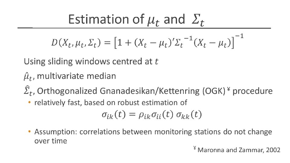
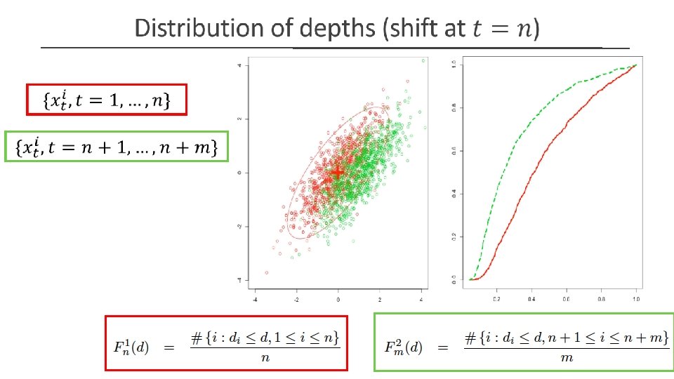
Depth of a multivariate observation

The standardized Kolmogorov-Smirnov statistic

Block Bootstrap

Multiple breakpoints – Binary trees

Growing the tree. First step

Growing the tree. Second step

The finest partition (saturated tree) 7 breakpoints 8 segments

Pruning of the tree 3 breakpoints 4 segments

Final step

Regional Model Simulated Data* Four time series of daily minimum temperature, Argentina were generated Time span: 1981 to 2100 (120 years = 43929 days) We introduced 4 inhomogeneities 1. 2. 3. 4. Grid point 1, day 8, 000, mean shift = + 0. 5 °C Grid point 2, day 16, 000, mean shift = - 0. 5 °C Grid point 3, day 24, 000, mean shift = + 0. 5 °C Grid point 4, day 30, 000, mean shift = - 0. 5 °C *Rossby Center Regional Climate model (Swedish Meteorological and Hydrological Institute) simulates the main atmospheric variables for the South American region on a daily basis

Growing the tree

Detected breakpoints

Identifying the responsible station

Performance of the methods Multivariate time series were generated from regional climate models under different scenarios • Number of stations in the influence set and distances between them • Kind and magnitude of changes in distributions 5 breakpoints at random locations (separated at least 5 years), i. e. , 6 different regimes were artificially created, mean expected duration 20 years. Procedure is repeated 20 times to allow for 100 breakpoints to be detected in the same conditions Performance of the method was evaluated using AUC (ROC curves) Performance increases with information (# stations, closeness of stations) and size/length of the change.

Conclusions We have developed a methodology that • • Is automated, does not require expert knowledge input Uses information from multiple stations simultaneously Detects several breakpoints per station Evaluates the significance of the breakpoint Identifies the kind of change/inhomogeneity (mean, variance, etc. ) Makes no distributional assumptions Accounts for dependence in the climatic data Is based on robust estimators Codes developed in R

Remarks The methodology can be used with for any continuous variable like atmospheric pressure, humidity or heliophany. Detecting breakpoints in precipitation TS requires an adaptation 1. precipitation is less spatially -and temporally- smooth than temperature 2. precipitation data encloses two pieces of information, whether the event rain had occurred (rain yes/no) and given that it occurred, its intensity

Thank you!