A 2 Level Maths Statistics 2 for Edexcel

A 2 -Level Maths: Statistics 2 for Edexcel S 2. 3 Continuous distributions This icon indicates the slide contains activities created in Flash. These activities are not editable. For more detailed instructions, see the Getting Started presentation. 1 of 39 © Boardworks Ltd 2006

Continuous uniform distribution Contents Continuous uniform distribution Approximating the binomial using a normal Approximating the Poisson using a normal 2 of 39 © Boardworks Ltd 2006

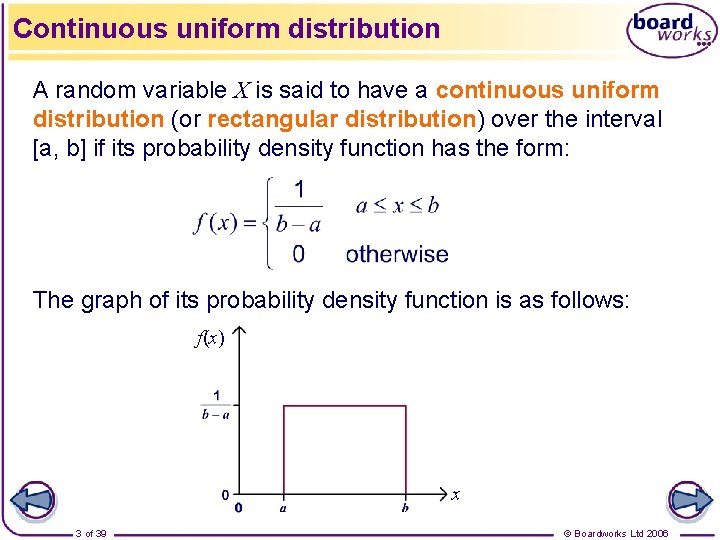
Continuous uniform distribution A random variable X is said to have a continuous uniform distribution (or rectangular distribution) over the interval [a, b] if its probability density function has the form: The graph of its probability density function is as follows: f(x) x 3 of 39 © Boardworks Ltd 2006

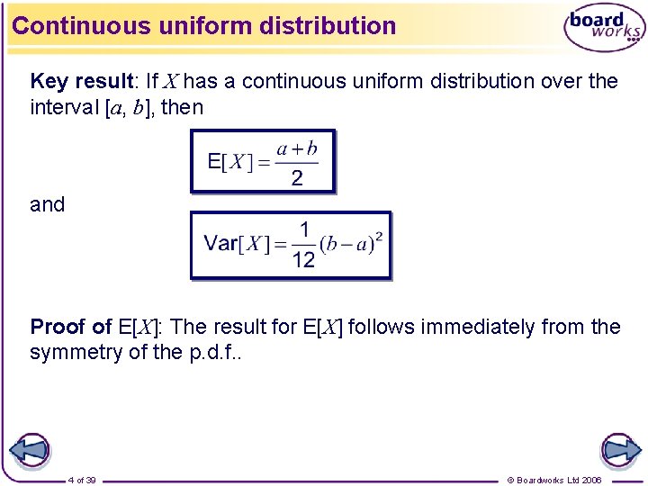
Continuous uniform distribution Key result: If X has a continuous uniform distribution over the interval [a, b], then and Proof of E[X]: The result for E[X] follows immediately from the symmetry of the p. d. f. . 4 of 39 © Boardworks Ltd 2006

Continuous uniform distribution Proof of Var[X]: So, 5 of 39 © Boardworks Ltd 2006

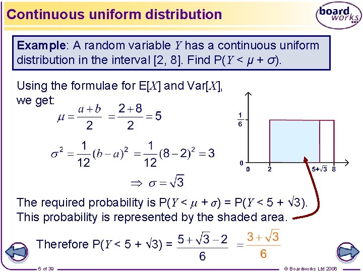
Continuous uniform distribution Example: A random variable Y has a continuous uniform distribution in the interval [2, 8]. Find P(Y < μ + σ). Using the formulae for E[X] and Var[X], we get: The required probability is P(Y < μ + σ) = P(Y < 5 + √ 3). This probability is represented by the shaded area. Therefore P(Y < 5 + √ 3) = 6 of 39 © Boardworks Ltd 2006

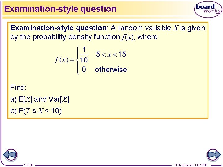
Examination-style question: A random variable X is given by the probability density function f (x), where Find: a) E[X] and Var[X] b) P(7 ≤ X < 10) 7 of 39 © Boardworks Ltd 2006

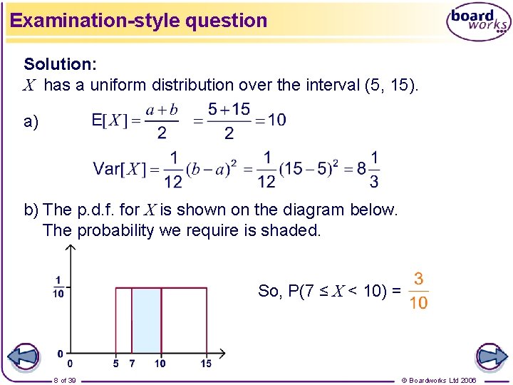
Examination-style question Solution: X has a uniform distribution over the interval (5, 15). a) b) The p. d. f. for X is shown on the diagram below. The probability we require is shaded. So, P(7 ≤ X < 10) = 8 of 39 © Boardworks Ltd 2006

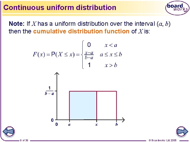
Continuous uniform distribution Note: If X has a uniform distribution over the interval (a, b) then the cumulative distribution function of X is: 9 of 39 © Boardworks Ltd 2006

Approximating the binomial using a normal Contents Continuous uniform distribution Approximating the binomial using a normal Approximating the Poisson using a normal 10 of 39 © Boardworks Ltd 2006

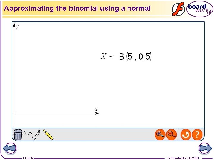
Approximating the binomial using a normal 11 of 39 © Boardworks Ltd 2006

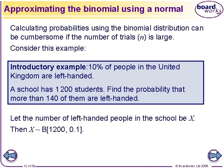
Approximating the binomial using a normal Calculating probabilities using the binomial distribution can be cumbersome if the number of trials (n) is large. Consider this example: Introductory example: 10% of people in the United Kingdom are left-handed. A school has 1 200 students. Find the probability that more than 140 of them are left-handed. Let the number of left-handed people in the school be X. Then X ~ B[1200, 0. 1]. 12 of 39 © Boardworks Ltd 2006

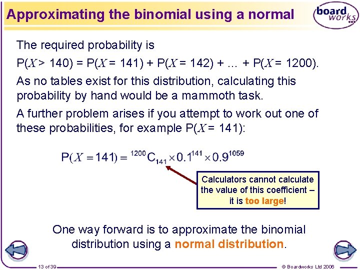
Approximating the binomial using a normal The required probability is P(X > 140) = P(X = 141) + P(X = 142) + … + P(X = 1200). As no tables exist for this distribution, calculating this probability by hand would be a mammoth task. A further problem arises if you attempt to work out one of these probabilities, for example P(X = 141): Calculators cannot calculate the value of this coefficient – it is too large! One way forward is to approximate the binomial distribution using a normal distribution. 13 of 39 © Boardworks Ltd 2006

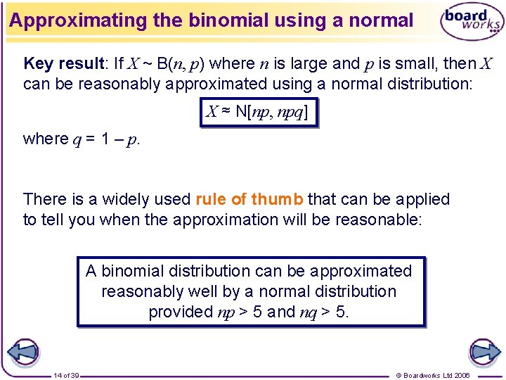
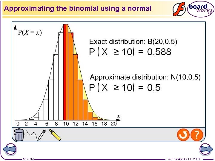
Approximating the binomial using a normal Key result: If X ~ B(n, p) where n is large and p is small, then X can be reasonably approximated using a normal distribution: X ≈ N[np, npq] where q = 1 – p. There is a widely used rule of thumb that can be applied to tell you when the approximation will be reasonable: A binomial distribution can be approximated reasonably well by a normal distribution provided np > 5 and nq > 5. 14 of 39 © Boardworks Ltd 2006

Approximating the binomial using a normal 15 of 39 © Boardworks Ltd 2006

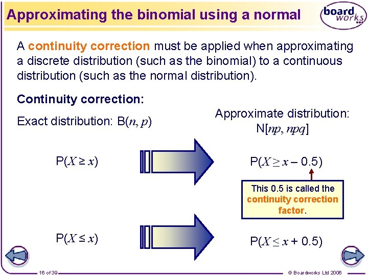
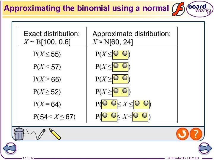
Approximating the binomial using a normal A continuity correction must be applied when approximating a discrete distribution (such as the binomial) to a continuous distribution (such as the normal distribution). Continuity correction: Exact distribution: B(n, p) P(X ≥ x) Approximate distribution: N[np, npq] P(X ≥ x – 0. 5) This 0. 5 is called the continuity correction factor. P(X ≤ x) 16 of 39 P(X ≤ x + 0. 5) © Boardworks Ltd 2006

Approximating the binomial using a normal 17 of 39 © Boardworks Ltd 2006

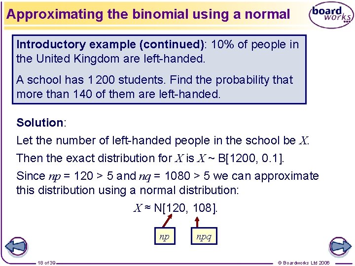
Approximating the binomial using a normal Introductory example (continued): 10% of people in the United Kingdom are left-handed. A school has 1 200 students. Find the probability that more than 140 of them are left-handed. Solution: Let the number of left-handed people in the school be X. Then the exact distribution for X is X ~ B[1200, 0. 1]. Since np = 120 > 5 and nq = 1080 > 5 we can approximate this distribution using a normal distribution: X ≈ N[120, 108]. np 18 of 39 npq © Boardworks Ltd 2006

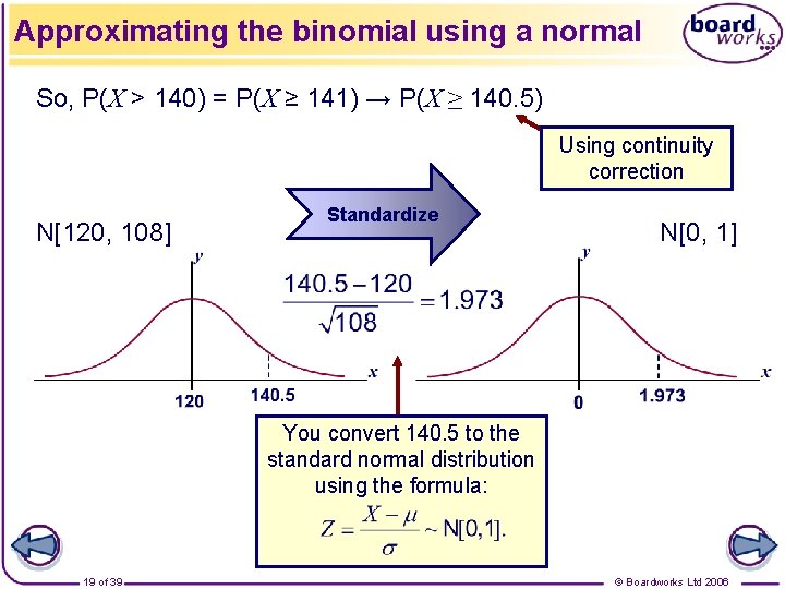
Approximating the binomial using a normal So, P(X > 140) = P(X ≥ 141) → P(X ≥ 140. 5) Using continuity correction N[120, 108] Standardize N[0, 1] You convert 140. 5 to the standard normal distribution using the formula: 19 of 39 © Boardworks Ltd 2006

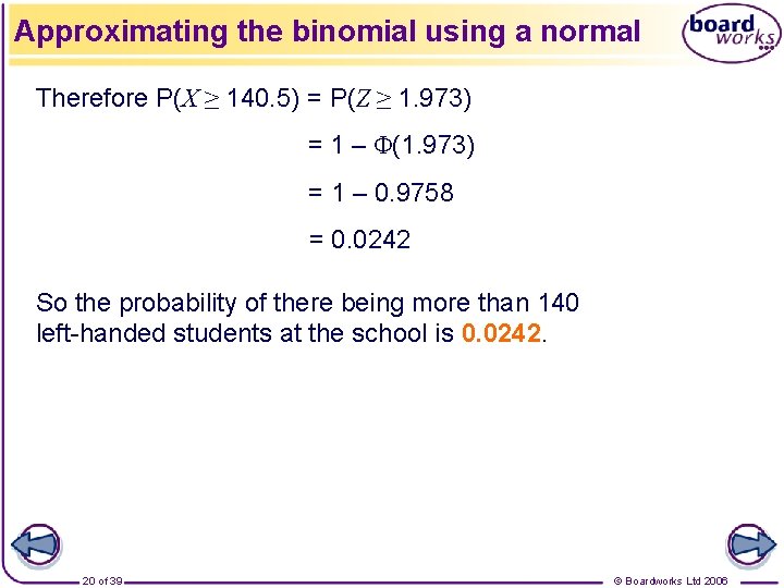
Approximating the binomial using a normal Therefore P(X ≥ 140. 5) = P(Z ≥ 1. 973) = 1 – Φ(1. 973) = 1 – 0. 9758 = 0. 0242 So the probability of there being more than 140 left-handed students at the school is 0. 0242. 20 of 39 © Boardworks Ltd 2006

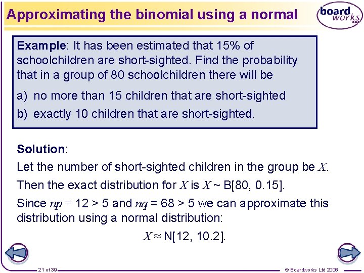
Approximating the binomial using a normal Example: It has been estimated that 15% of schoolchildren are short-sighted. Find the probability that in a group of 80 schoolchildren there will be a) no more than 15 children that are short-sighted b) exactly 10 children that are short-sighted. Solution: Let the number of short-sighted children in the group be X. Then the exact distribution for X is X ~ B[80, 0. 15]. Since np = 12 > 5 and nq = 68 > 5 we can approximate this distribution using a normal distribution: X ≈ N[12, 10. 2]. 21 of 39 © Boardworks Ltd 2006

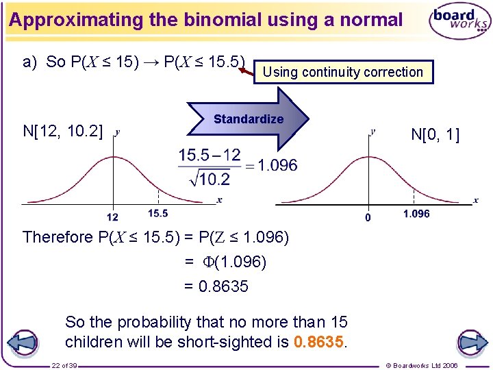
Approximating the binomial using a normal a) So P(X ≤ 15) → P(X ≤ 15. 5) N[12, 10. 2] Using continuity correction Standardize N[0, 1] Therefore P(X ≤ 15. 5) = P(Z ≤ 1. 096) = Φ(1. 096) = 0. 8635 So the probability that no more than 15 children will be short-sighted is 0. 8635. 22 of 39 © Boardworks Ltd 2006

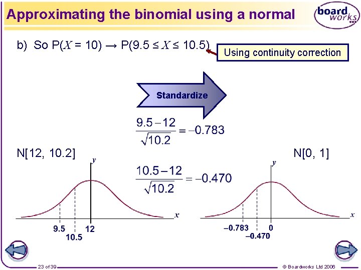
Approximating the binomial using a normal b) So P(X = 10) → P(9. 5 ≤ X ≤ 10. 5) Using continuity correction Standardize N[12, 10. 2] 23 of 39 N[0, 1] © Boardworks Ltd 2006

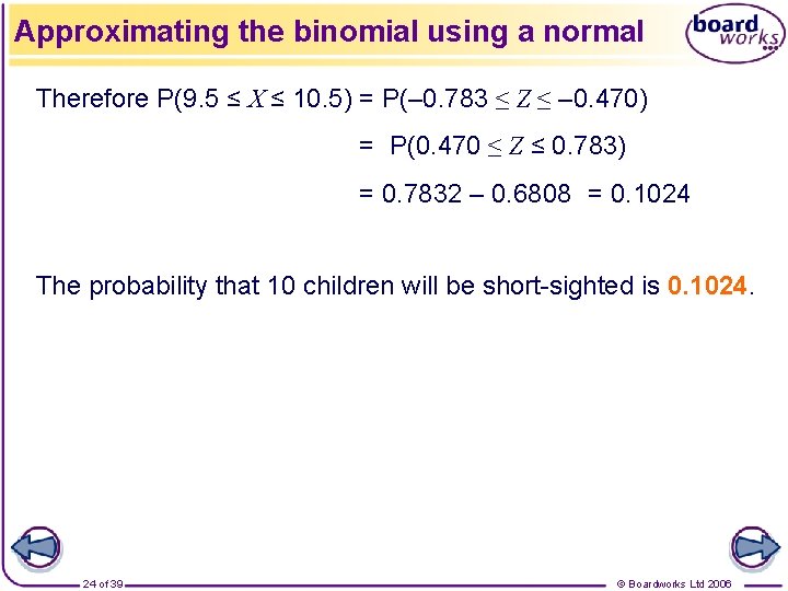
Approximating the binomial using a normal Therefore P(9. 5 ≤ X ≤ 10. 5) = P(– 0. 783 ≤ Z ≤ – 0. 470) = P(0. 470 ≤ Z ≤ 0. 783) = 0. 7832 – 0. 6808 = 0. 1024 The probability that 10 children will be short-sighted is 0. 1024. 24 of 39 © Boardworks Ltd 2006

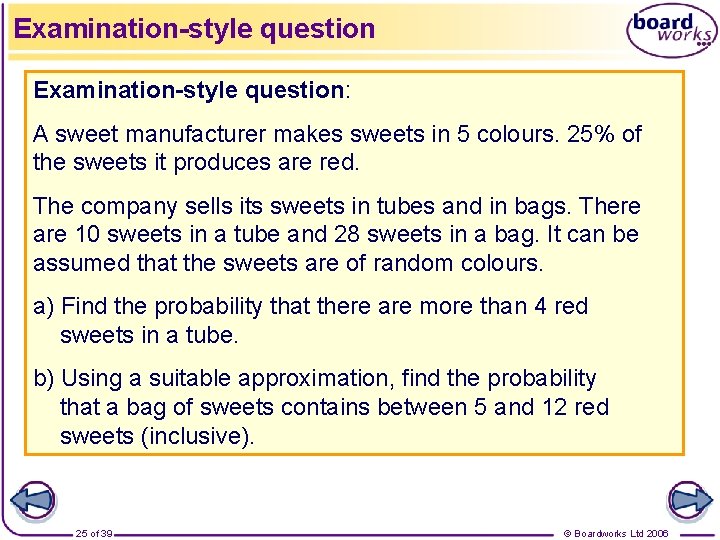
Examination-style question: A sweet manufacturer makes sweets in 5 colours. 25% of the sweets it produces are red. The company sells its sweets in tubes and in bags. There are 10 sweets in a tube and 28 sweets in a bag. It can be assumed that the sweets are of random colours. a) Find the probability that there are more than 4 red sweets in a tube. b) Using a suitable approximation, find the probability that a bag of sweets contains between 5 and 12 red sweets (inclusive). 25 of 39 © Boardworks Ltd 2006

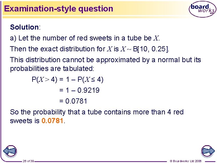
Examination-style question Solution: a) Let the number of red sweets in a tube be X. Then the exact distribution for X is X ~ B[10, 0. 25]. This distribution cannot be approximated by a normal but its probabilities are tabulated: P(X > 4) = 1 – P(X ≤ 4) = 1 – 0. 9219 = 0. 0781 So the probability that a tube contains more than 4 red sweets is 0. 0781. 26 of 39 © Boardworks Ltd 2006

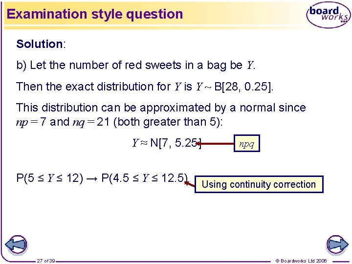
Examination style question Solution: b) Let the number of red sweets in a bag be Y. Then the exact distribution for Y is Y ~ B[28, 0. 25]. This distribution can be approximated by a normal since np = 7 and nq = 21 (both greater than 5): Y ≈ N[7, 5. 25] P(5 ≤ Y ≤ 12) → P(4. 5 ≤ Y ≤ 12. 5) 27 of 39 npq Using continuity correction © Boardworks Ltd 2006

Examination style question Standardize N[7, 5. 25] N[0, 1] Therefore P(4. 5 ≤ Y ≤ 12. 5) = P(– 1. 091 ≤ Z ≤ 2. 400) = P(Z ≤ 2. 400) – P(Z ≤ – 1. 091) = Φ(2. 400) – (1 – Φ(1. 091)) = 0. 9918 – (1 – 0. 8623) = 0. 8541 So the probability that a bag will contain between 5 and 12 red sweets is 0. 8541. 28 of 39 © Boardworks Ltd 2006

Approximating the Poisson using a normal Contents Continuous uniform distribution Approximating the binomial using a normal Approximating the Poisson using a normal 29 of 39 © Boardworks Ltd 2006

Approximating the Poisson using a normal 30 of 39 © Boardworks Ltd 2006

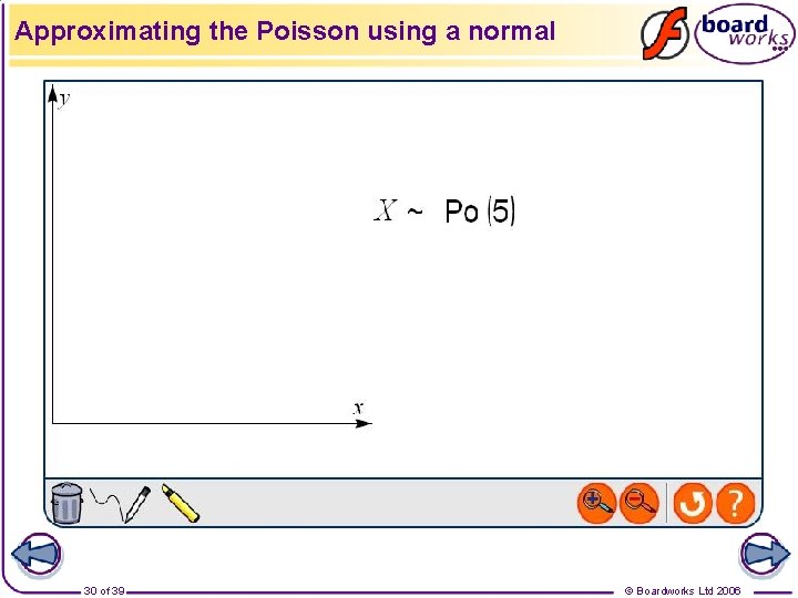
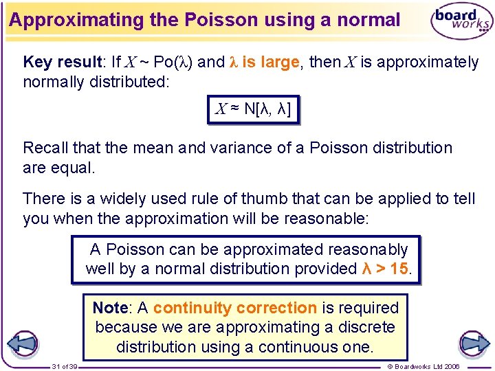
Approximating the Poisson using a normal Key result: If X ~ Po(λ) and λ is large, then X is approximately normally distributed: X ≈ N[λ, λ] Recall that the mean and variance of a Poisson distribution are equal. There is a widely used rule of thumb that can be applied to tell you when the approximation will be reasonable: A Poisson can be approximated reasonably well by a normal distribution provided λ > 15. Note: A continuity correction is required because we are approximating a discrete distribution using a continuous one. 31 of 39 © Boardworks Ltd 2006

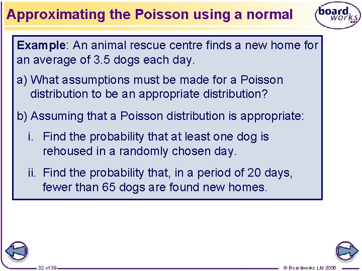
Approximating the Poisson using a normal Example: An animal rescue centre finds a new home for an average of 3. 5 dogs each day. a) What assumptions must be made for a Poisson distribution to be an appropriate distribution? b) Assuming that a Poisson distribution is appropriate: i. Find the probability that at least one dog is rehoused in a randomly chosen day. ii. Find the probability that, in a period of 20 days, fewer than 65 dogs are found new homes. 32 of 39 © Boardworks Ltd 2006

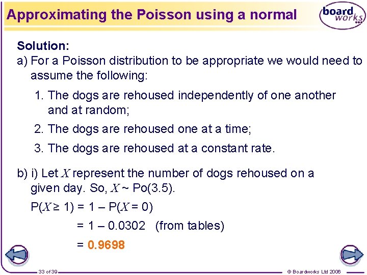
Approximating the Poisson using a normal Solution: a) For a Poisson distribution to be appropriate we would need to assume the following: 1. The dogs are rehoused independently of one another and at random; 2. The dogs are rehoused one at a time; 3. The dogs are rehoused at a constant rate. b) i) Let X represent the number of dogs rehoused on a given day. So, X ~ Po(3. 5). P(X ≥ 1) = 1 – P(X = 0) = 1 – 0. 0302 (from tables) = 0. 9698 33 of 39 © Boardworks Ltd 2006

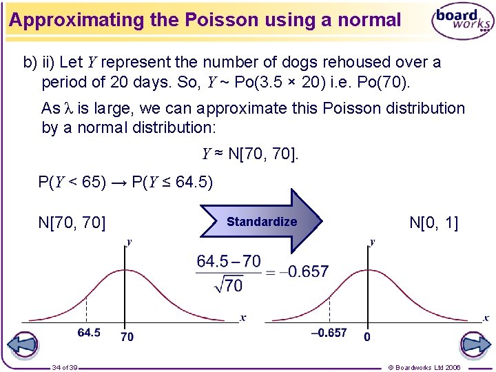
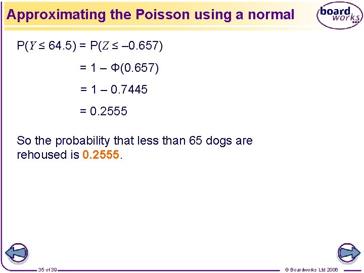
Approximating the Poisson using a normal b) ii) Let Y represent the number of dogs rehoused over a period of 20 days. So, Y ~ Po(3. 5 × 20) i. e. Po(70). As λ is large, we can approximate this Poisson distribution by a normal distribution: Y ≈ N[70, 70]. P(Y < 65) → P(Y ≤ 64. 5) N[70, 70] 34 of 39 Standardize N[0, 1] © Boardworks Ltd 2006

Approximating the Poisson using a normal P(Y ≤ 64. 5) = P(Z ≤ – 0. 657) = 1 – Φ(0. 657) = 1 – 0. 7445 = 0. 2555 So the probability that less than 65 dogs are rehoused is 0. 2555. 35 of 39 © Boardworks Ltd 2006

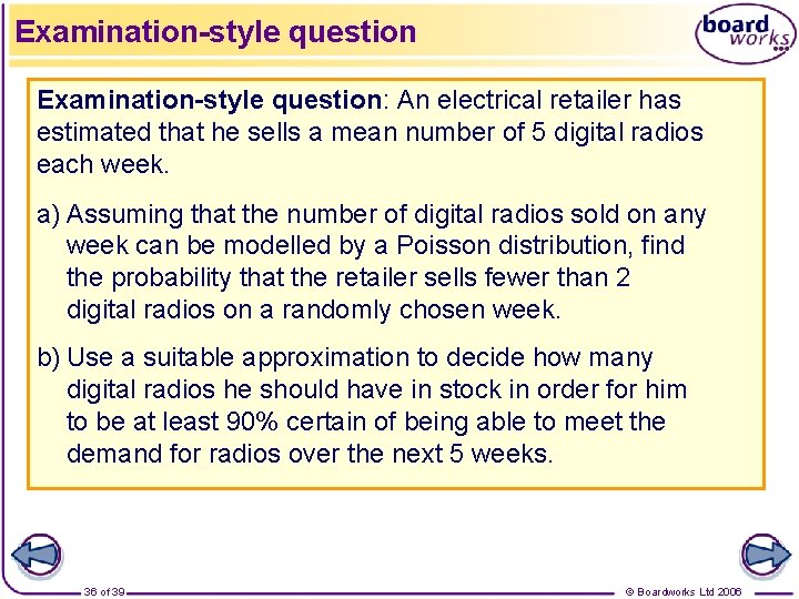
Examination-style question: An electrical retailer has estimated that he sells a mean number of 5 digital radios each week. a) Assuming that the number of digital radios sold on any week can be modelled by a Poisson distribution, find the probability that the retailer sells fewer than 2 digital radios on a randomly chosen week. b) Use a suitable approximation to decide how many digital radios he should have in stock in order for him to be at least 90% certain of being able to meet the demand for radios over the next 5 weeks. 36 of 39 © Boardworks Ltd 2006

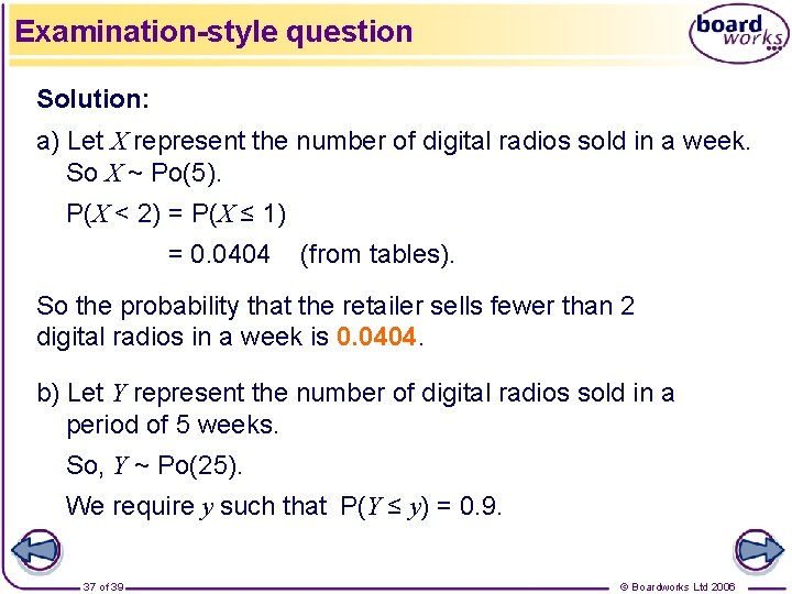
Examination-style question Solution: a) Let X represent the number of digital radios sold in a week. So X ~ Po(5). P(X < 2) = P(X ≤ 1) = 0. 0404 (from tables). So the probability that the retailer sells fewer than 2 digital radios in a week is 0. 0404. b) Let Y represent the number of digital radios sold in a period of 5 weeks. So, Y ~ Po(25). We require y such that P(Y ≤ y) = 0. 9. 37 of 39 © Boardworks Ltd 2006

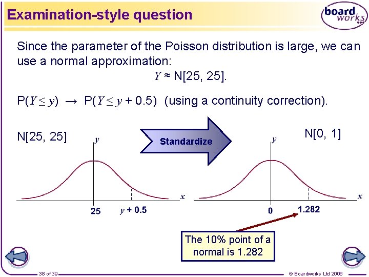
Examination-style question Since the parameter of the Poisson distribution is large, we can use a normal approximation: Y ≈ N[25, 25]. P(Y ≤ y) → P(Y ≤ y + 0. 5) (using a continuity correction). N[25, 25] Standardize N[0, 1] The 10% point of a normal is 1. 282 38 of 39 © Boardworks Ltd 2006

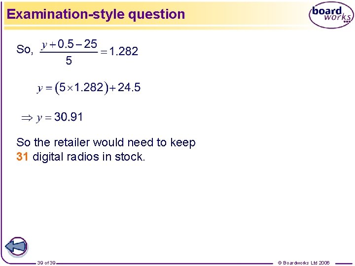
Examination-style question So, So the retailer would need to keep 31 digital radios in stock. 39 of 39 © Boardworks Ltd 2006