A 2 Level Maths Statistics 2 for Edexcel

A 2 -Level Maths: Statistics 2 for Edexcel S 2. 3 Continuous distributions These icons indicate that teacher’s notes or useful web addresses are available in the Notes Page. This icon indicates the slide contains activities created in Flash. These activities are not editable. For more detailed instructions, see the Getting Started presentation. 1 of 39 © Boardworks Ltd 2006

Continuous uniform distribution Contents Continuous uniform distribution Approximating the binomial using a normal Approximating the Poisson using a normal 2 of 39 © Boardworks Ltd 2006

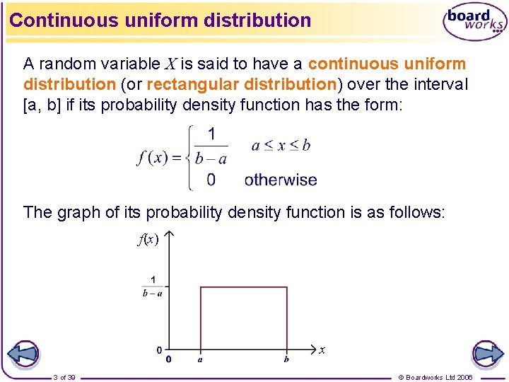
Continuous uniform distribution A random variable X is said to have a continuous uniform distribution (or rectangular distribution) over the interval [a, b] if its probability density function has the form: The graph of its probability density function is as follows: f(x) x 3 of 39 © Boardworks Ltd 2006

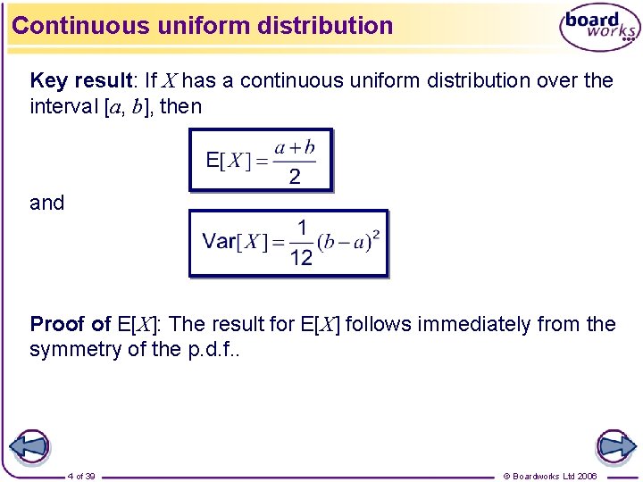
Continuous uniform distribution Key result: If X has a continuous uniform distribution over the interval [a, b], then and Proof of E[X]: The result for E[X] follows immediately from the symmetry of the p. d. f. . 4 of 39 © Boardworks Ltd 2006

Continuous uniform distribution Proof of Var[X]: So, 5 of 39 © Boardworks Ltd 2006

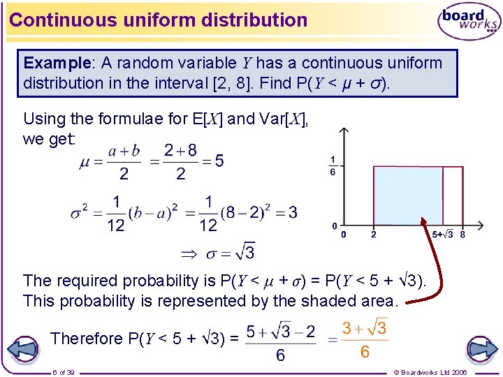
Continuous uniform distribution Example: A random variable Y has a continuous uniform distribution in the interval [2, 8]. Find P(Y < μ + σ). Using the formulae for E[X] and Var[X], we get: The required probability is P(Y < μ + σ) = P(Y < 5 + √ 3). This probability is represented by the shaded area. Therefore P(Y < 5 + √ 3) = 6 of 39 © Boardworks Ltd 2006

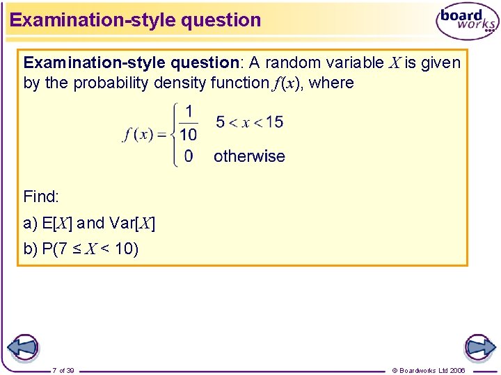
Examination-style question: A random variable X is given by the probability density function f (x), where Find: a) E[X] and Var[X] b) P(7 ≤ X < 10) 7 of 39 © Boardworks Ltd 2006

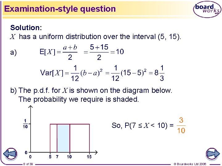
Examination-style question Solution: X has a uniform distribution over the interval (5, 15). a) b) The p. d. f. for X is shown on the diagram below. The probability we require is shaded. So, P(7 ≤ X < 10) = 8 of 39 © Boardworks Ltd 2006

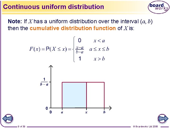
Continuous uniform distribution Note: If X has a uniform distribution over the interval (a, b) then the cumulative distribution function of X is: 9 of 39 © Boardworks Ltd 2006

Approximating the binomial using a normal Contents Continuous uniform distribution Approximating the binomial using a normal Approximating the Poisson using a normal 10 of 39 © Boardworks Ltd 2006

Approximating the binomial using a normal 11 of 39 © Boardworks Ltd 2006

Approximating the binomial using a normal Calculating probabilities using the binomial distribution can be cumbersome if the number of trials (n) is large. Consider this example: Introductory example: 10% of people in the United Kingdom are left-handed. A school has 1 200 students. Find the probability that more than 140 of them are left-handed. Let the number of left-handed people in the school be X. Then X ~ B[1200, 0. 1]. 12 of 39 © Boardworks Ltd 2006

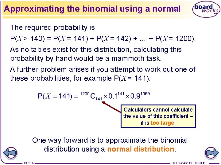
Approximating the binomial using a normal The required probability is P(X > 140) = P(X = 141) + P(X = 142) + … + P(X = 1200). As no tables exist for this distribution, calculating this probability by hand would be a mammoth task. A further problem arises if you attempt to work out one of these probabilities, for example P(X = 141): Calculators cannot calculate the value of this coefficient – it is too large! One way forward is to approximate the binomial distribution using a normal distribution. 13 of 39 © Boardworks Ltd 2006

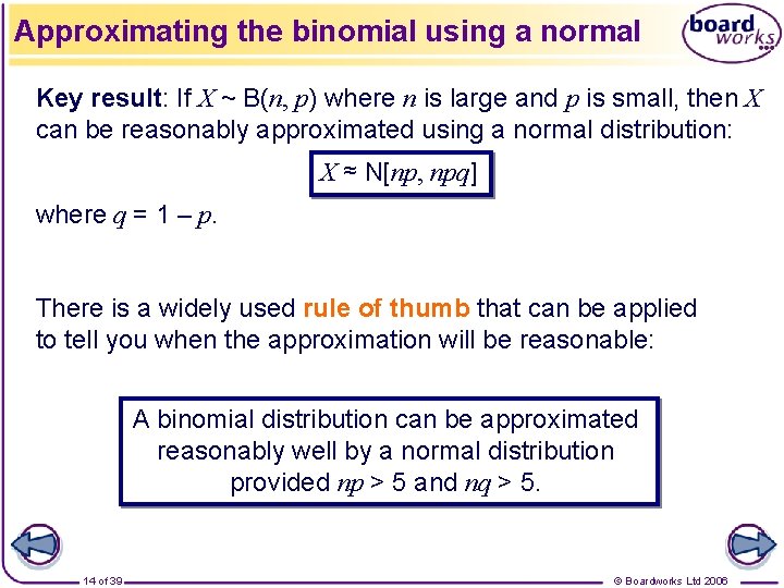
Approximating the binomial using a normal Key result: If X ~ B(n, p) where n is large and p is small, then X can be reasonably approximated using a normal distribution: X ≈ N[np, npq] where q = 1 – p. There is a widely used rule of thumb that can be applied to tell you when the approximation will be reasonable: A binomial distribution can be approximated reasonably well by a normal distribution provided np > 5 and nq > 5. 14 of 39 © Boardworks Ltd 2006

Approximating the binomial using a normal 15 of 39 © Boardworks Ltd 2006

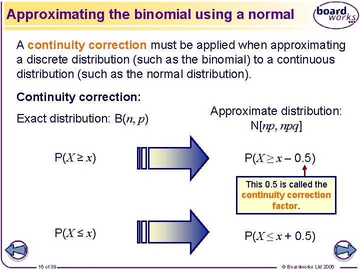
Approximating the binomial using a normal A continuity correction must be applied when approximating a discrete distribution (such as the binomial) to a continuous distribution (such as the normal distribution). Continuity correction: Exact distribution: B(n, p) P(X ≥ x) Approximate distribution: N[np, npq] P(X ≥ x – 0. 5) This 0. 5 is called the continuity correction factor. P(X ≤ x) 16 of 39 P(X ≤ x + 0. 5) © Boardworks Ltd 2006

Approximating the binomial using a normal 17 of 39 © Boardworks Ltd 2006

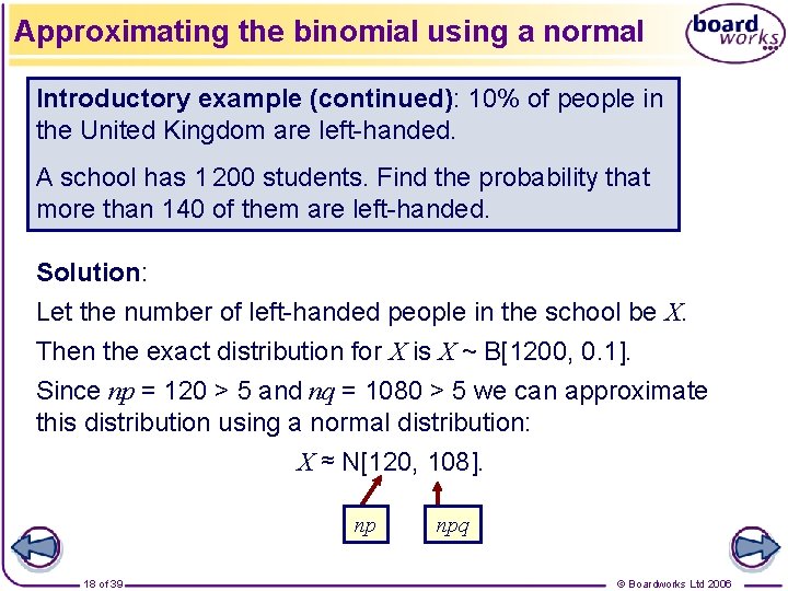
Approximating the binomial using a normal Introductory example (continued): 10% of people in the United Kingdom are left-handed. A school has 1 200 students. Find the probability that more than 140 of them are left-handed. Solution: Let the number of left-handed people in the school be X. Then the exact distribution for X is X ~ B[1200, 0. 1]. Since np = 120 > 5 and nq = 1080 > 5 we can approximate this distribution using a normal distribution: X ≈ N[120, 108]. np 18 of 39 npq © Boardworks Ltd 2006

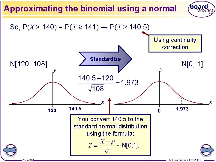
Approximating the binomial using a normal So, P(X > 140) = P(X ≥ 141) → P(X ≥ 140. 5) Using continuity correction N[120, 108] Standardize N[0, 1] You convert 140. 5 to the standard normal distribution using the formula: 19 of 39 © Boardworks Ltd 2006

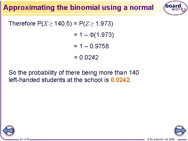
Approximating the binomial using a normal Therefore P(X ≥ 140. 5) = P(Z ≥ 1. 973) = 1 – Φ(1. 973) = 1 – 0. 9758 = 0. 0242 So the probability of there being more than 140 left-handed students at the school is 0. 0242. 20 of 39 © Boardworks Ltd 2006

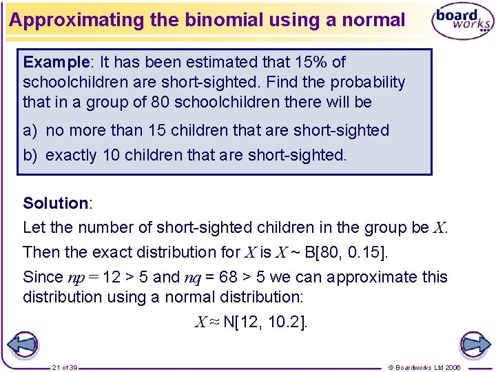
Approximating the binomial using a normal Example: It has been estimated that 15% of schoolchildren are short-sighted. Find the probability that in a group of 80 schoolchildren there will be a) no more than 15 children that are short-sighted b) exactly 10 children that are short-sighted. Solution: Let the number of short-sighted children in the group be X. Then the exact distribution for X is X ~ B[80, 0. 15]. Since np = 12 > 5 and nq = 68 > 5 we can approximate this distribution using a normal distribution: X ≈ N[12, 10. 2]. 21 of 39 © Boardworks Ltd 2006

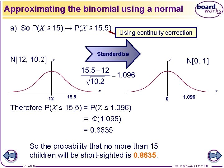
Approximating the binomial using a normal a) So P(X ≤ 15) → P(X ≤ 15. 5) N[12, 10. 2] Using continuity correction Standardize N[0, 1] Therefore P(X ≤ 15. 5) = P(Z ≤ 1. 096) = Φ(1. 096) = 0. 8635 So the probability that no more than 15 children will be short-sighted is 0. 8635. 22 of 39 © Boardworks Ltd 2006

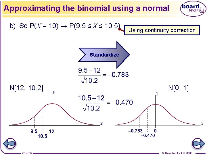
Approximating the binomial using a normal b) So P(X = 10) → P(9. 5 ≤ X ≤ 10. 5) Using continuity correction Standardize N[12, 10. 2] 23 of 39 N[0, 1] © Boardworks Ltd 2006

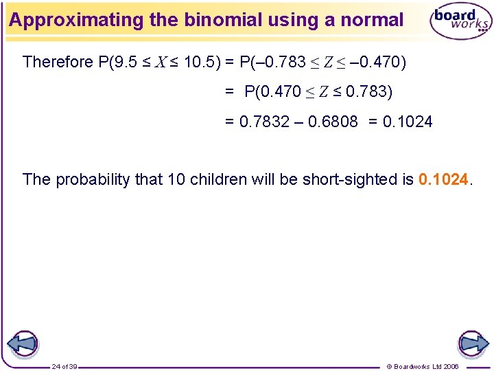
Approximating the binomial using a normal Therefore P(9. 5 ≤ X ≤ 10. 5) = P(– 0. 783 ≤ Z ≤ – 0. 470) = P(0. 470 ≤ Z ≤ 0. 783) = 0. 7832 – 0. 6808 = 0. 1024 The probability that 10 children will be short-sighted is 0. 1024. 24 of 39 © Boardworks Ltd 2006

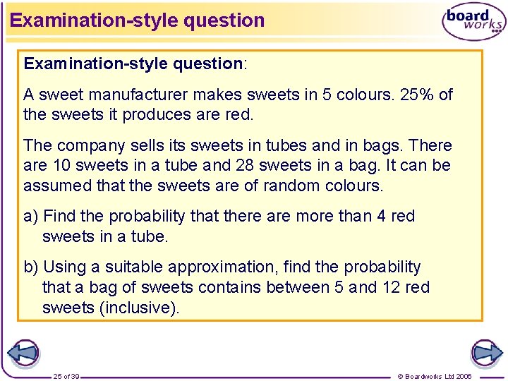
Examination-style question: A sweet manufacturer makes sweets in 5 colours. 25% of the sweets it produces are red. The company sells its sweets in tubes and in bags. There are 10 sweets in a tube and 28 sweets in a bag. It can be assumed that the sweets are of random colours. a) Find the probability that there are more than 4 red sweets in a tube. b) Using a suitable approximation, find the probability that a bag of sweets contains between 5 and 12 red sweets (inclusive). 25 of 39 © Boardworks Ltd 2006

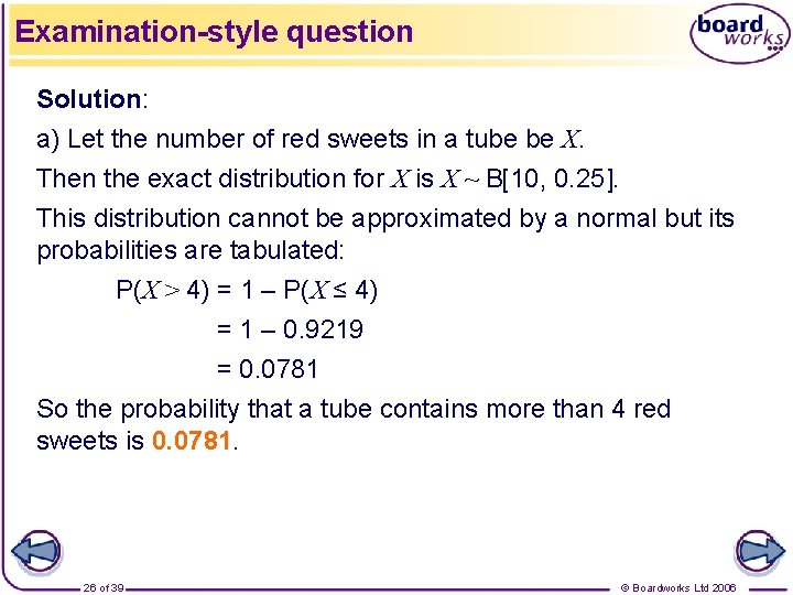
Examination-style question Solution: a) Let the number of red sweets in a tube be X. Then the exact distribution for X is X ~ B[10, 0. 25]. This distribution cannot be approximated by a normal but its probabilities are tabulated: P(X > 4) = 1 – P(X ≤ 4) = 1 – 0. 9219 = 0. 0781 So the probability that a tube contains more than 4 red sweets is 0. 0781. 26 of 39 © Boardworks Ltd 2006

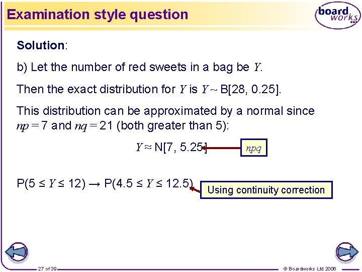
Examination style question Solution: b) Let the number of red sweets in a bag be Y. Then the exact distribution for Y is Y ~ B[28, 0. 25]. This distribution can be approximated by a normal since np = 7 and nq = 21 (both greater than 5): Y ≈ N[7, 5. 25] P(5 ≤ Y ≤ 12) → P(4. 5 ≤ Y ≤ 12. 5) 27 of 39 npq Using continuity correction © Boardworks Ltd 2006

Examination style question Standardize N[7, 5. 25] N[0, 1] Therefore P(4. 5 ≤ Y ≤ 12. 5) = P(– 1. 091 ≤ Z ≤ 2. 400) = P(Z ≤ 2. 400) – P(Z ≤ – 1. 091) = Φ(2. 400) – (1 – Φ(1. 091)) = 0. 9918 – (1 – 0. 8623) = 0. 8541 So the probability that a bag will contain between 5 and 12 red sweets is 0. 8541. 28 of 39 © Boardworks Ltd 2006

Approximating the Poisson using a normal Contents Continuous uniform distribution Approximating the binomial using a normal Approximating the Poisson using a normal 29 of 39 © Boardworks Ltd 2006

Approximating the Poisson using a normal 30 of 39 © Boardworks Ltd 2006

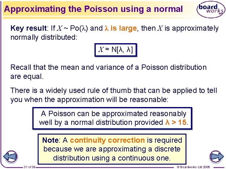
Approximating the Poisson using a normal Key result: If X ~ Po(λ) and λ is large, then X is approximately normally distributed: X ≈ N[λ, λ] Recall that the mean and variance of a Poisson distribution are equal. There is a widely used rule of thumb that can be applied to tell you when the approximation will be reasonable: A Poisson can be approximated reasonably well by a normal distribution provided λ > 15. Note: A continuity correction is required because we are approximating a discrete distribution using a continuous one. 31 of 39 © Boardworks Ltd 2006

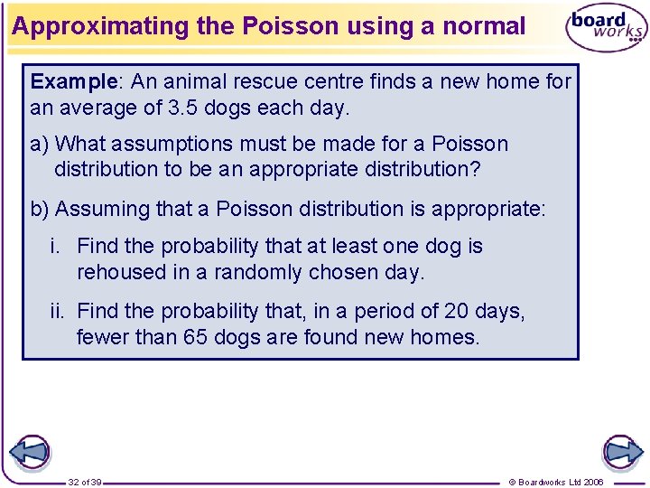
Approximating the Poisson using a normal Example: An animal rescue centre finds a new home for an average of 3. 5 dogs each day. a) What assumptions must be made for a Poisson distribution to be an appropriate distribution? b) Assuming that a Poisson distribution is appropriate: i. Find the probability that at least one dog is rehoused in a randomly chosen day. ii. Find the probability that, in a period of 20 days, fewer than 65 dogs are found new homes. 32 of 39 © Boardworks Ltd 2006

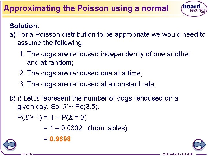
Approximating the Poisson using a normal Solution: a) For a Poisson distribution to be appropriate we would need to assume the following: 1. The dogs are rehoused independently of one another and at random; 2. The dogs are rehoused one at a time; 3. The dogs are rehoused at a constant rate. b) i) Let X represent the number of dogs rehoused on a given day. So, X ~ Po(3. 5). P(X ≥ 1) = 1 – P(X = 0) = 1 – 0. 0302 (from tables) = 0. 9698 33 of 39 © Boardworks Ltd 2006

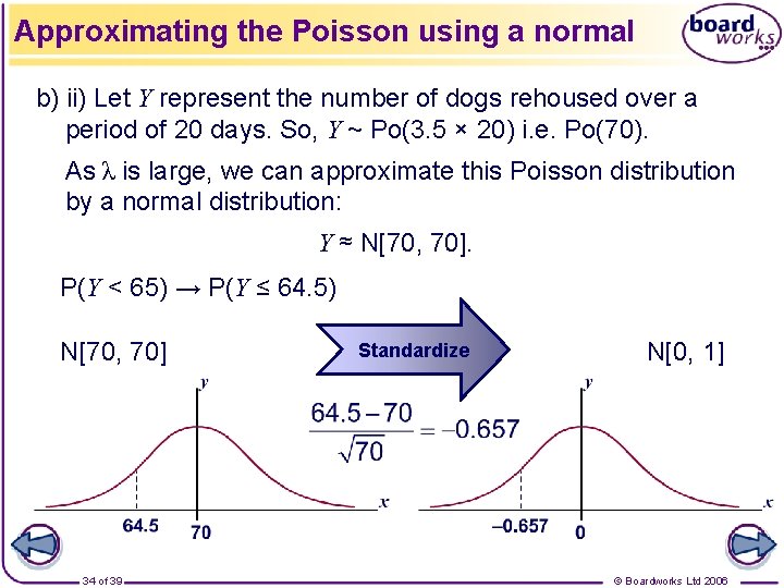
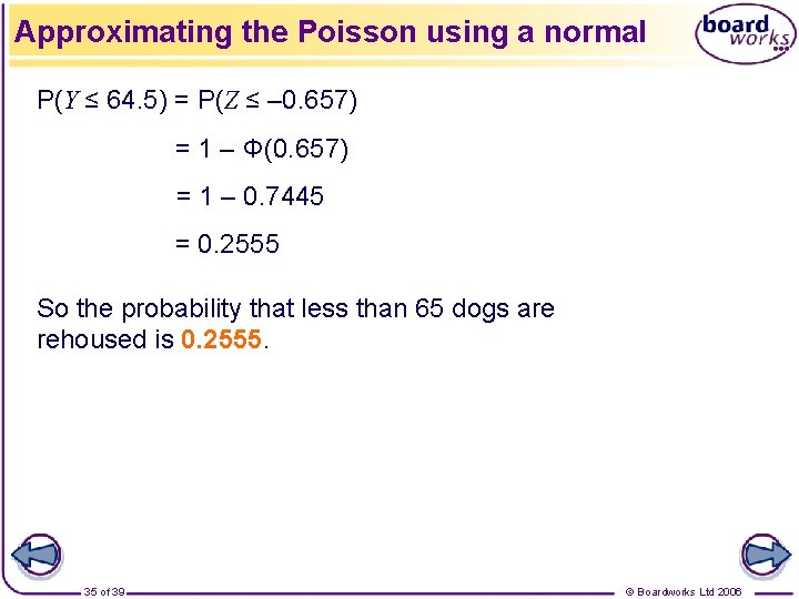
Approximating the Poisson using a normal b) ii) Let Y represent the number of dogs rehoused over a period of 20 days. So, Y ~ Po(3. 5 × 20) i. e. Po(70). As λ is large, we can approximate this Poisson distribution by a normal distribution: Y ≈ N[70, 70]. P(Y < 65) → P(Y ≤ 64. 5) N[70, 70] 34 of 39 Standardize N[0, 1] © Boardworks Ltd 2006

Approximating the Poisson using a normal P(Y ≤ 64. 5) = P(Z ≤ – 0. 657) = 1 – Φ(0. 657) = 1 – 0. 7445 = 0. 2555 So the probability that less than 65 dogs are rehoused is 0. 2555. 35 of 39 © Boardworks Ltd 2006

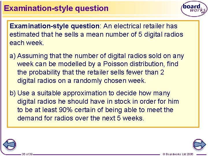
Examination-style question: An electrical retailer has estimated that he sells a mean number of 5 digital radios each week. a) Assuming that the number of digital radios sold on any week can be modelled by a Poisson distribution, find the probability that the retailer sells fewer than 2 digital radios on a randomly chosen week. b) Use a suitable approximation to decide how many digital radios he should have in stock in order for him to be at least 90% certain of being able to meet the demand for radios over the next 5 weeks. 36 of 39 © Boardworks Ltd 2006

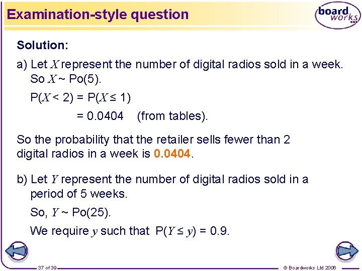
Examination-style question Solution: a) Let X represent the number of digital radios sold in a week. So X ~ Po(5). P(X < 2) = P(X ≤ 1) = 0. 0404 (from tables). So the probability that the retailer sells fewer than 2 digital radios in a week is 0. 0404. b) Let Y represent the number of digital radios sold in a period of 5 weeks. So, Y ~ Po(25). We require y such that P(Y ≤ y) = 0. 9. 37 of 39 © Boardworks Ltd 2006

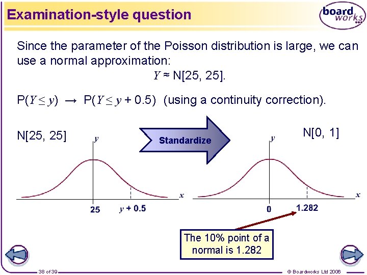
Examination-style question Since the parameter of the Poisson distribution is large, we can use a normal approximation: Y ≈ N[25, 25]. P(Y ≤ y) → P(Y ≤ y + 0. 5) (using a continuity correction). N[25, 25] Standardize N[0, 1] The 10% point of a normal is 1. 282 38 of 39 © Boardworks Ltd 2006

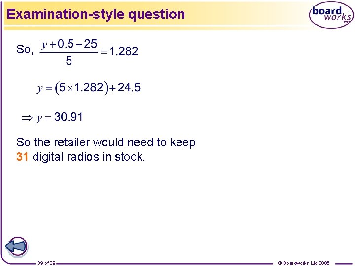
Examination-style question So, So the retailer would need to keep 31 digital radios in stock. 39 of 39 © Boardworks Ltd 2006