3 Applications of the Derivative Copyright Cengage Learning

3 Applications of the Derivative Copyright © Cengage Learning. All rights reserved. 1

3. 3 Concavity and the Second-Derivative Test Copyright © Cengage Learning. All rights reserved.

Objectives Determine the intervals on which the graphs of functions are concave upward or concave downward. Find the points of inflection of the graphs of functions. Use the Second-Derivative Test to find the relative extrema of functions. Find the points of diminishing returns of input-output models. 3

Concavity 4

Concavity You already know that locating the intervals over which a function f increases or decreases helps to describe its graph. In this section, you will see that locating the intervals on which f (the derivative of f) increases or decreases can determine where the graph of f is curving upward or curving downward. 5

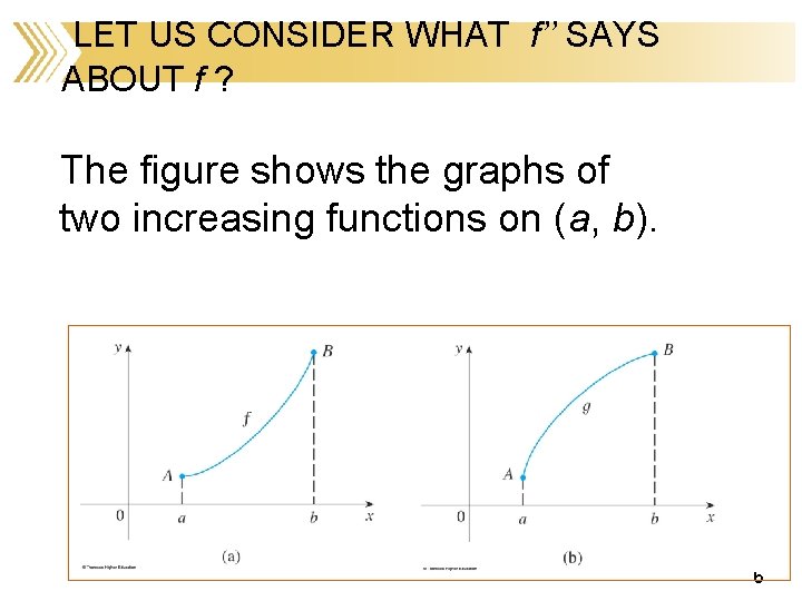
LET US CONSIDER WHAT f’’ SAYS ABOUT f ? The figure shows the graphs of two increasing functions on (a, b). 6

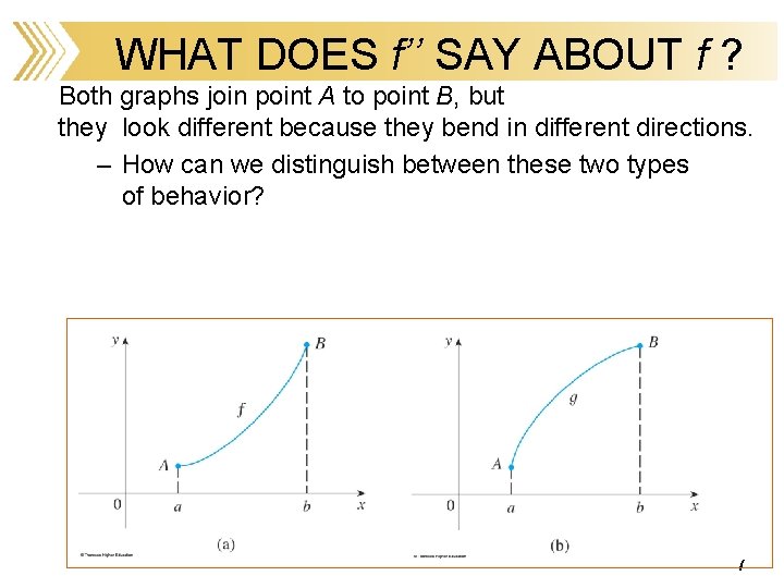
WHAT DOES f’’ SAY ABOUT f ? Both graphs join point A to point B, but they look different because they bend in different directions. – How can we distinguish between these two types of behavior? 7

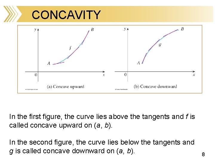
CONCAVITY In the first figure, the curve lies above the tangents and f is called concave upward on (a, b). In the second figure, the curve lies below the tangents and g is called concave downward on (a, b). 8

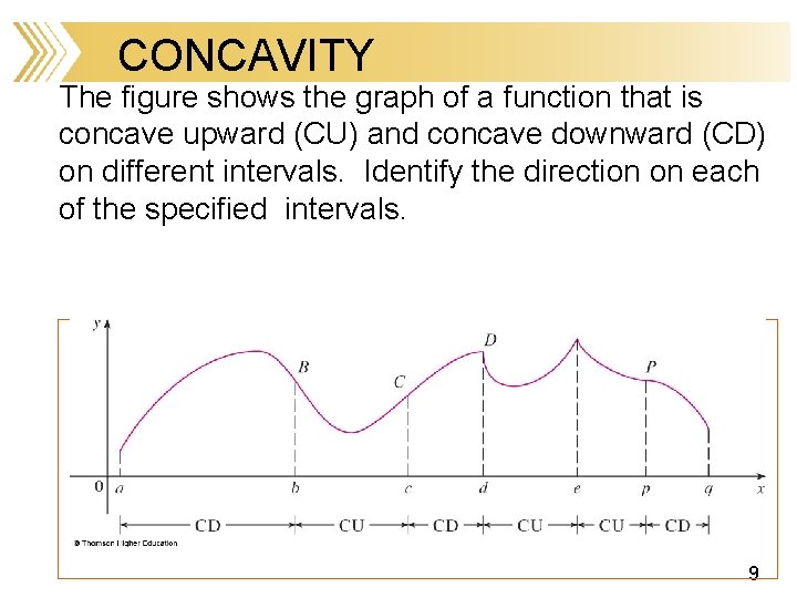
CONCAVITY The figure shows the graph of a function that is concave upward (CU) and concave downward (CD) on different intervals. Identify the direction on each of the specified intervals. 9

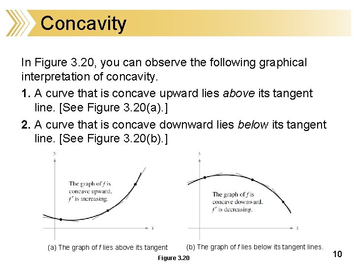
Concavity In Figure 3. 20, you can observe the following graphical interpretation of concavity. 1. A curve that is concave upward lies above its tangent line. [See Figure 3. 20(a). ] 2. A curve that is concave downward lies below its tangent line. [See Figure 3. 20(b). ] (a) The graph of f lies above its tangent (b) The graph of f lies below its tangent lines. Figure 3. 20 10

CONCAVITY Let’s see how the second derivative helps determine the intervals of concavity. 11

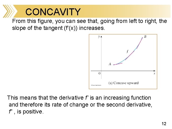
CONCAVITY From this figure, you can see that, going from left to right, the slope of the tangent (f’(x)) increases. This means that the derivative f’ is an increasing function and therefore its rate of change or the second derivative, f” , is positive. 12

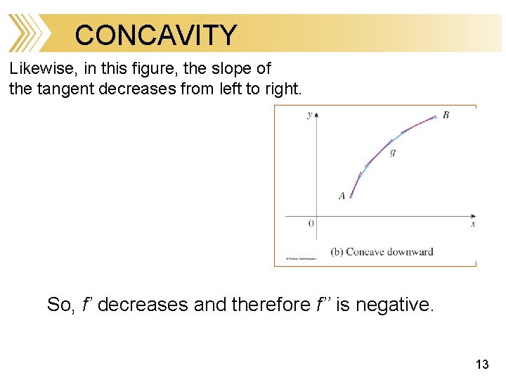
CONCAVITY Likewise, in this figure, the slope of the tangent decreases from left to right. So, f’ decreases and therefore f’’ is negative. 13

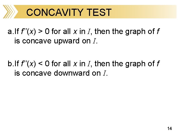
CONCAVITY TEST a. If f’’(x) > 0 for all x in I, then the graph of f is concave upward on I. b. If f’’(x) < 0 for all x in I, then the graph of f is concave downward on I. 14

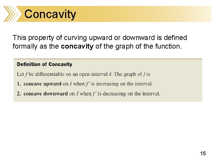
Concavity This property of curving upward or downward is defined formally as the concavity of the graph of the function. 15

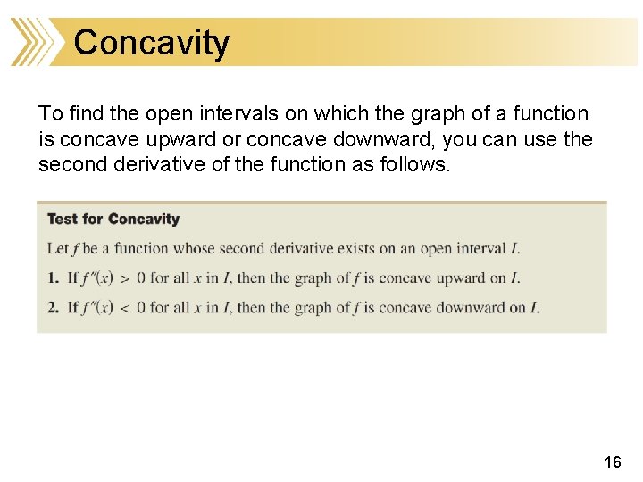
Concavity To find the open intervals on which the graph of a function is concave upward or concave downward, you can use the second derivative of the function as follows. 16

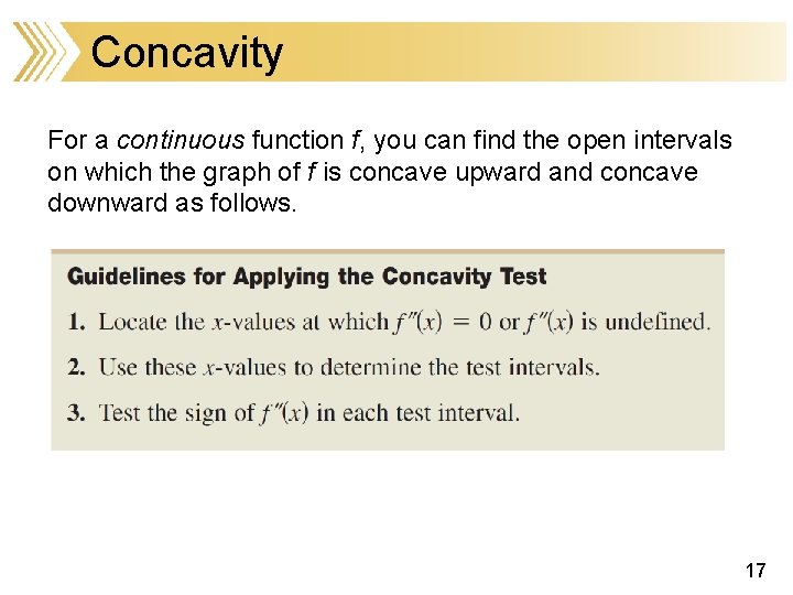
Concavity For a continuous function f, you can find the open intervals on which the graph of f is concave upward and concave downward as follows. 17

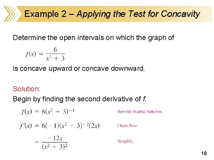
Example 2 – Applying the Test for Concavity Determine the open intervals on which the graph of is concave upward or concave downward. Solution: Begin by finding the second derivative of f. 18

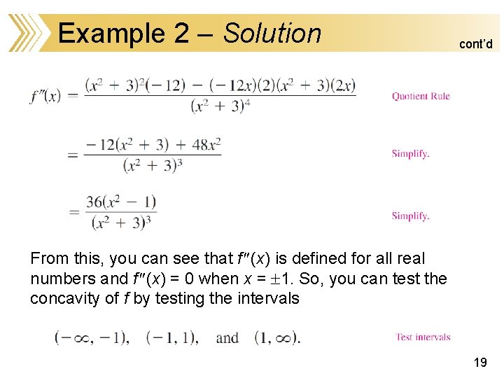
Example 2 – Solution cont’d From this, you can see that f (x) is defined for all real numbers and f (x) = 0 when x = 1. So, you can test the concavity of f by testing the intervals 19

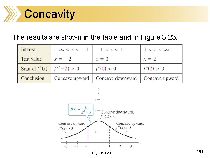
Concavity The results are shown in the table and in Figure 3. 23 20

Points of Inflection 21

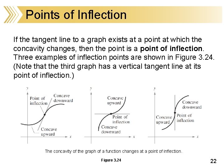
Points of Inflection If the tangent line to a graph exists at a point at which the concavity changes, then the point is a point of inflection. Three examples of inflection points are shown in Figure 3. 24. (Note that the third graph has a vertical tangent line at its point of inflection. ) The concavity of the graph of a function changes at a point of inflection. Figure 3. 24 22

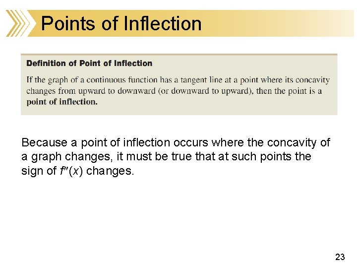
Points of Inflection Because a point of inflection occurs where the concavity of a graph changes, it must be true that at such points the sign of f (x) changes. 23

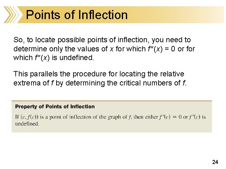
Points of Inflection So, to locate possible points of inflection, you need to determine only the values of x for which f (x) = 0 or for which f (x) is undefined. This parallels the procedure for locating the relative extrema of f by determining the critical numbers of f. 24

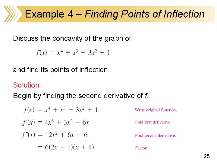
Example 4 – Finding Points of Inflection Discuss the concavity of the graph of and find its points of inflection. Solution: Begin by finding the second derivative of f. 25

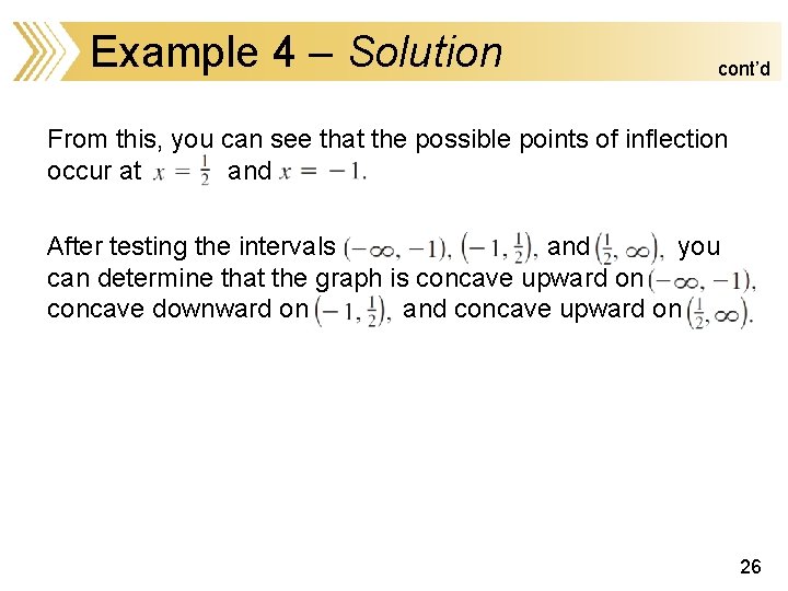
Example 4 – Solution cont’d From this, you can see that the possible points of inflection occur at and After testing the intervals and you can determine that the graph is concave upward on concave downward on and concave upward on 26

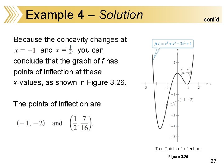
Example 4 – Solution cont’d Because the concavity changes at and you can conclude that the graph of f has points of inflection at these x-values, as shown in Figure 3. 26. The points of inflection are Two Points of Inflection Figure 3. 26 27

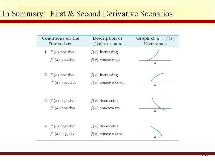
In Summary: First & Second Derivative Scenarios 28

The Second-Derivative Test 29

The Second-Derivative Test The second derivative can be used to perform a simple test for relative minima and relative maxima. If f is a function such that f (c) = 0 and the graph of f is concave upward at x = c, then f (c) is a relative minimum of f. 30

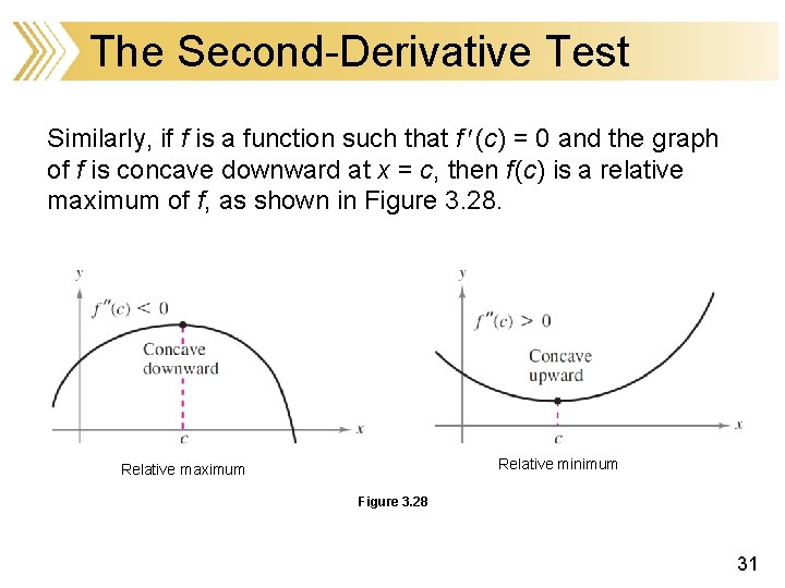
The Second-Derivative Test Similarly, if f is a function such that f (c) = 0 and the graph of f is concave downward at x = c, then f (c) is a relative maximum of f, as shown in Figure 3. 28. Relative minimum Relative maximum Figure 3. 28 31

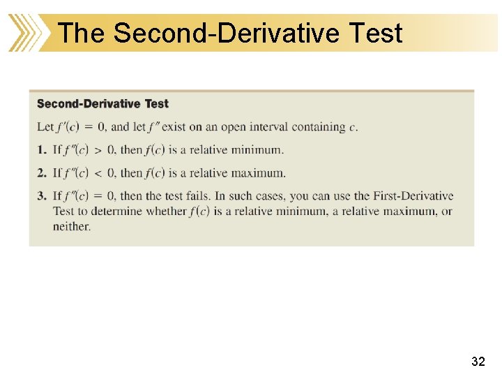
The Second-Derivative Test 32

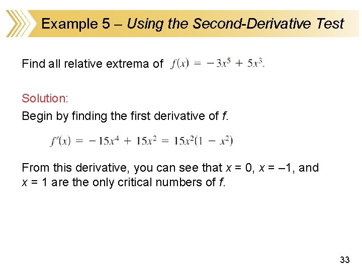
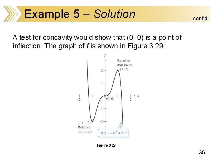
Example 5 – Using the Second-Derivative Test Find all relative extrema of Solution: Begin by finding the first derivative of f. From this derivative, you can see that x = 0, x = – 1, and x = 1 are the only critical numbers of f. 33

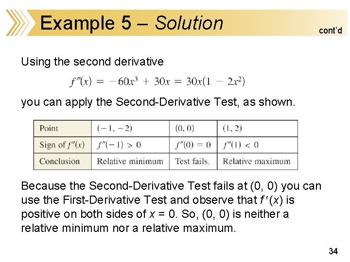
Example 5 – Solution cont’d Using the second derivative you can apply the Second-Derivative Test, as shown. Because the Second-Derivative Test fails at (0, 0) you can use the First-Derivative Test and observe that f (x) is positive on both sides of x = 0. So, (0, 0) is neither a relative minimum nor a relative maximum. 34

Example 5 – Solution cont’d A test for concavity would show that (0, 0) is a point of inflection. The graph of f is shown in Figure 3. 29 35

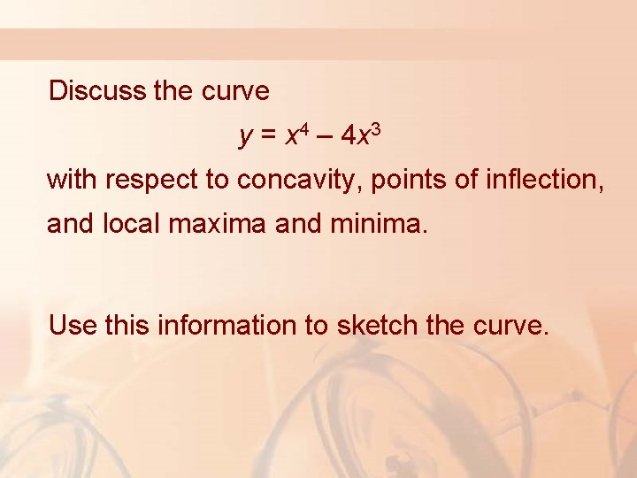
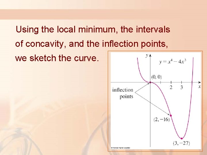
Discuss the curve y = x 4 – 4 x 3 with respect to concavity, points of inflection, and local maxima and minima. Use this information to sketch the curve.

Using the local minimum, the intervals of concavity, and the inflection points, we sketch the curve.

Application: Diminishing Returns 38

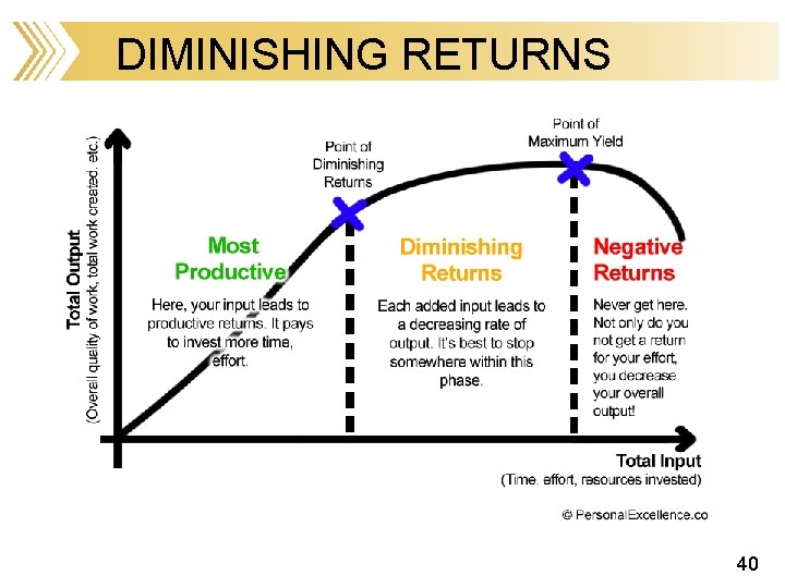
DIMINISHING RETURNS In economics, the inflection point of the profit or revenue functions is called the point of diminishing returns Before the inflection point, or point of diminishing returns, the rate of profit is increasing, while after it is decreasing. The inflection point is the point where it begins to get more difficult to increase profit. 39

DIMINISHING RETURNS 40

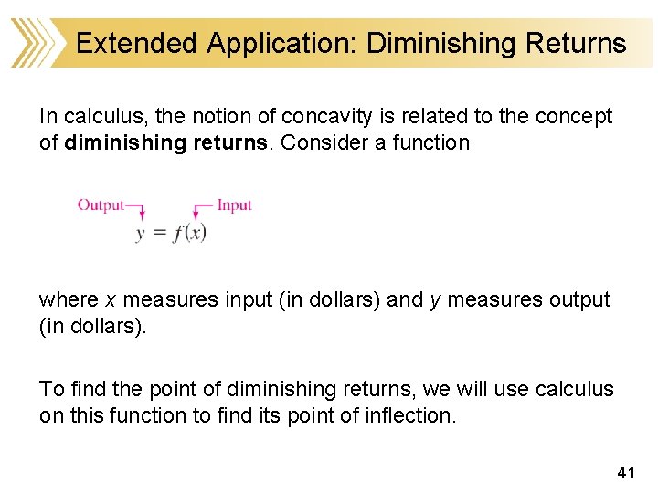
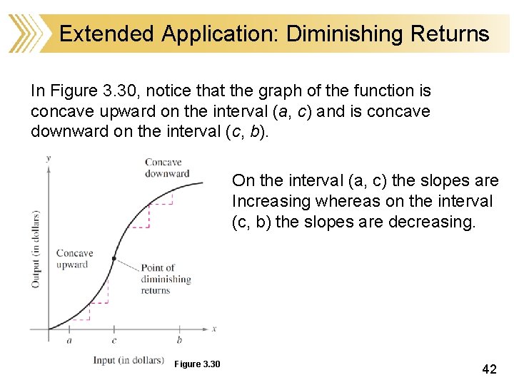
Extended Application: Diminishing Returns In calculus, the notion of concavity is related to the concept of diminishing returns. Consider a function where x measures input (in dollars) and y measures output (in dollars). To find the point of diminishing returns, we will use calculus on this function to find its point of inflection. 41

Extended Application: Diminishing Returns In Figure 3. 30, notice that the graph of the function is concave upward on the interval (a, c) and is concave downward on the interval (c, b). On the interval (a, c) the slopes are Increasing whereas on the interval (c, b) the slopes are decreasing. Figure 3. 30 42

Extended Application: Diminishing Returns On the interval (a, c), each additional dollar of input returns more than the previous input dollar. By contrast, on the interval (c, b) each additional dollar of input returns less than the previous input dollar. The point (c, f (c)) is called the point of diminishing returns. An increased investment beyond this point is usually considered a poor use of capital. 43

Extended Application: Diminishing Returns On the interval (a, c), each additional dollar of input returns more than the previous input dollar. By contrast, on the interval (c, b) each additional dollar of input returns less than the previous input dollar. The point (c, f (c)) is called the point of diminishing returns. An increased investment beyond this point is usually considered a poor use of capital. 44

Extended Application: Diminishing Returns On the interval (a, c), each additional dollar of input returns more than the previous input dollar. By contrast, on the interval (c, b) each additional dollar of input returns less than the previous input dollar. The point (c, f (c)) is called the point of diminishing returns. An increased investment beyond this point is usually considered a poor use of capital. 45

Extended Application: Diminishing Returns On the interval (a, c), each additional dollar of input returns more than the previous input dollar. By contrast, on the interval (c, b) each additional dollar of input returns less than the previous input dollar. The point (c, f (c)) is called the point of diminishing returns. An increased investment beyond this point is usually considered a poor use of capital. 46

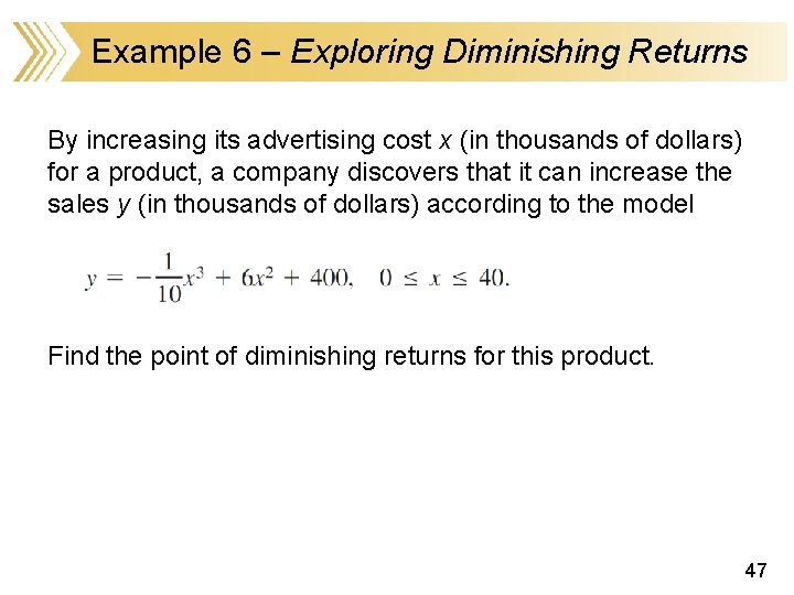
Example 6 – Exploring Diminishing Returns By increasing its advertising cost x (in thousands of dollars) for a product, a company discovers that it can increase the sales y (in thousands of dollars) according to the model Find the point of diminishing returns for this product. 47

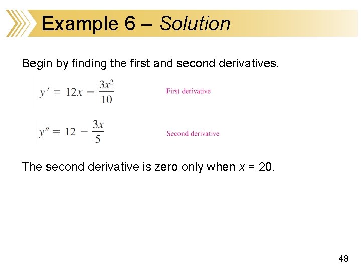
Example 6 – Solution Begin by finding the first and second derivatives. The second derivative is zero only when x = 20. 48

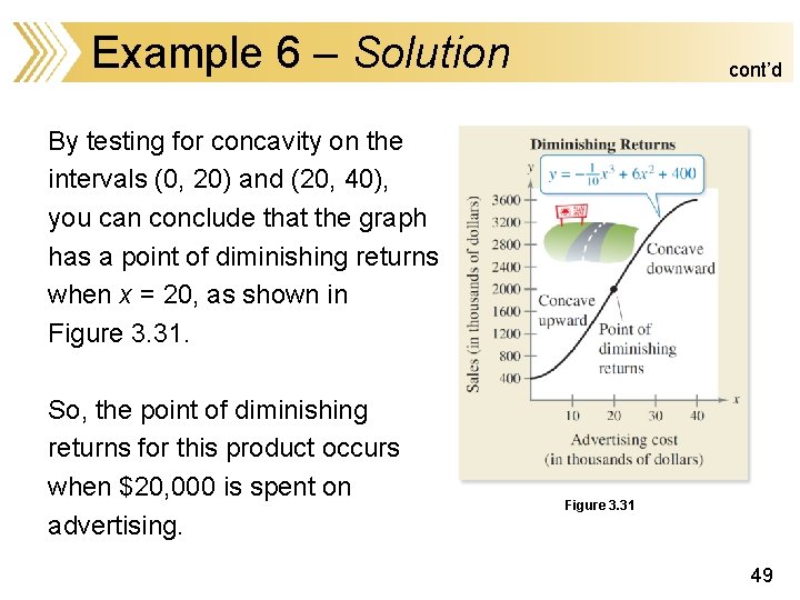
Example 6 – Solution cont’d By testing for concavity on the intervals (0, 20) and (20, 40), you can conclude that the graph has a point of diminishing returns when x = 20, as shown in Figure 3. 31. So, the point of diminishing returns for this product occurs when $20, 000 is spent on advertising. Figure 3. 31 49