Wojciech Gerson 1831 1901 Microeconomics Dali Laxton LECTURE

Wojciech Gerson (1831 -1901) Microeconomics Dali Laxton LECTURE 5 The Costs of Production Chapter 13

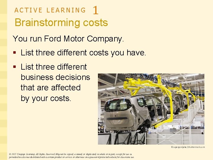
ACTIVE LEARNING 1 Brainstorming costs You run Ford Motor Company. § List three different costs you have. § List three different business decisions that are affected by your costs. ©supergenijalac/Shutterstock. com © 2015 Cengage Learning. All Rights Reserved. May not be copied, scanned, or duplicated, in whole or in part, except for use as permitted in a license distributed with a certain product or service or otherwise on a password-protected website for classroom use.

Lecture Today • What is a production function? What is marginal product? How are they related? • What are the various costs? How are they related to each other and to output? • How are costs different in the short run vs. the long run? • What are “economies of scale”? © 2015 Cengage Learning. All Rights Reserved. May not be copied, scanned, or duplicated, in whole or in part, except for use as permitted in a license distributed with a certain product or service or otherwise on a password-protected website for classroom use.

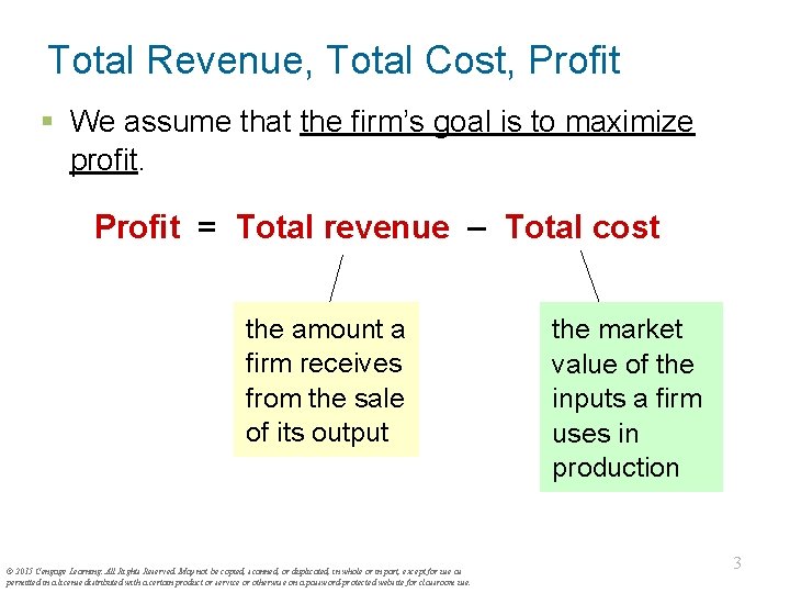
Total Revenue, Total Cost, Profit § We assume that the firm’s goal is to maximize profit. Profit = Total revenue – Total cost the amount a firm receives from the sale of its output © 2015 Cengage Learning. All Rights Reserved. May not be copied, scanned, or duplicated, in whole or in part, except for use as permitted in a license distributed with a certain product or service or otherwise on a password-protected website for classroom use. the market value of the inputs a firm uses in production 3

Costs: Explicit vs. Implicit § Explicit costs require an outlay of money, e. g. , paying wages to workers. § Implicit costs do not require a cash outlay, e. g. , the opportunity cost of the owner’s time. § Remember one of the Ten Principles: The cost of something is what you give up to get it. § This is true whether the costs are implicit or explicit. Both matter for firms’ decisions. © 2015 Cengage Learning. All Rights Reserved. May not be copied, scanned, or duplicated, in whole or in part, except for use as permitted in a license distributed with a certain product or service or otherwise on a password-protected website for classroom use. 4

Explicit vs. Implicit Costs: An Example You need $100, 000 to start your business. The interest rate is 5%. § Case 1: borrow $100, 000 § explicit cost = $5000 interest on loan § Case 2: use $40, 000 of your savings, borrow the other $60, 000 § explicit cost = $3000 (5%) interest on the loan § implicit cost = $2000 (5%) foregone interest you could have earned on your $40, 000. In both cases, total (exp + imp) costs are $5000. © 2015 Cengage Learning. All Rights Reserved. May not be copied, scanned, or duplicated, in whole or in part, except for use as permitted in a license distributed with a certain product or service or otherwise on a password-protected website for classroom use. 5

Economic Profit vs. Accounting Profit § Accounting profit = total revenue minus total explicit costs § Economic profit = total revenue minus total costs (including explicit and implicit costs) § Accounting profit ignores implicit costs, so it’s higher than economic profit. © 2015 Cengage Learning. All Rights Reserved. May not be copied, scanned, or duplicated, in whole or in part, except for use as permitted in a license distributed with a certain product or service or otherwise on a password-protected website for classroom use. 6

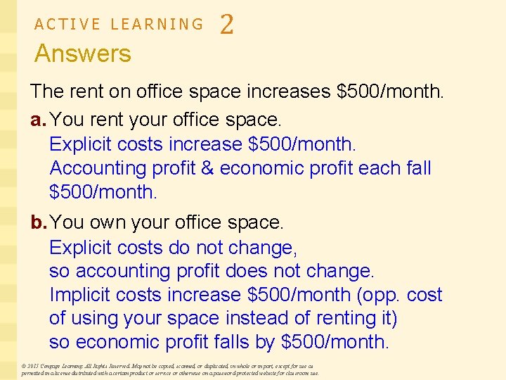
ACTIVE LEARNING 2 Economic profit vs. accounting profit The equilibrium rent on office space has just increased by $500/month. Determine the effects on accounting profit and economic profit if: a. you rent your office space b. you own your office space © 2015 Cengage Learning. All Rights Reserved. May not be copied, scanned, or duplicated, in whole or in part, except for use as permitted in a license distributed with a certain product or service or otherwise on a password-protected website for classroom use.

ACTIVE LEARNING Answers 2 The rent on office space increases $500/month. a. You rent your office space. Explicit costs increase $500/month. Accounting profit & economic profit each fall $500/month. b. You own your office space. Explicit costs do not change, so accounting profit does not change. Implicit costs increase $500/month (opp. cost of using your space instead of renting it) so economic profit falls by $500/month. © 2015 Cengage Learning. All Rights Reserved. May not be copied, scanned, or duplicated, in whole or in part, except for use as permitted in a license distributed with a certain product or service or otherwise on a password-protected website for classroom use.

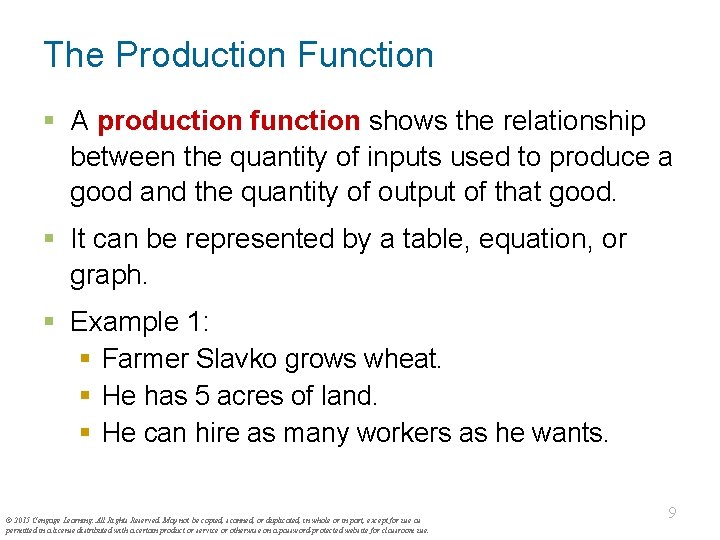
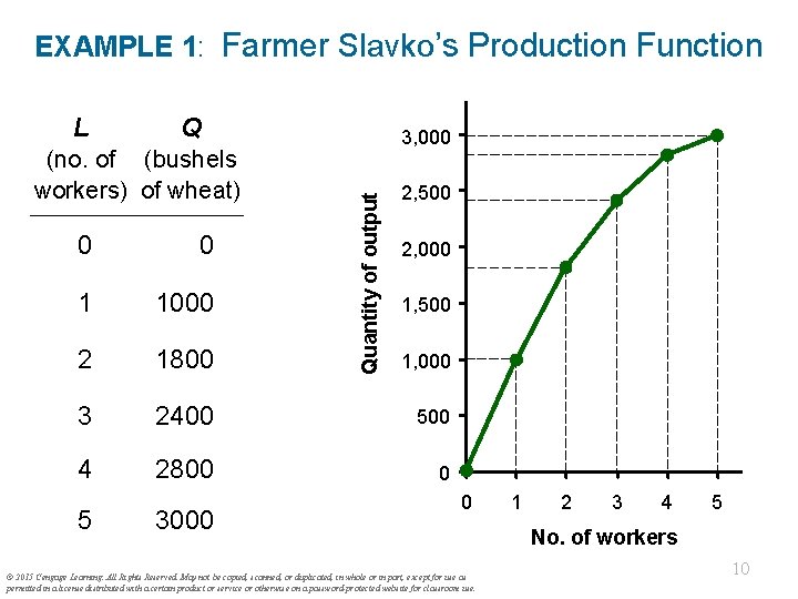
The Production Function § A production function shows the relationship between the quantity of inputs used to produce a good and the quantity of output of that good. § It can be represented by a table, equation, or graph. § Example 1: § Farmer Slavko grows wheat. § He has 5 acres of land. § He can hire as many workers as he wants. © 2015 Cengage Learning. All Rights Reserved. May not be copied, scanned, or duplicated, in whole or in part, except for use as permitted in a license distributed with a certain product or service or otherwise on a password-protected website for classroom use. 9

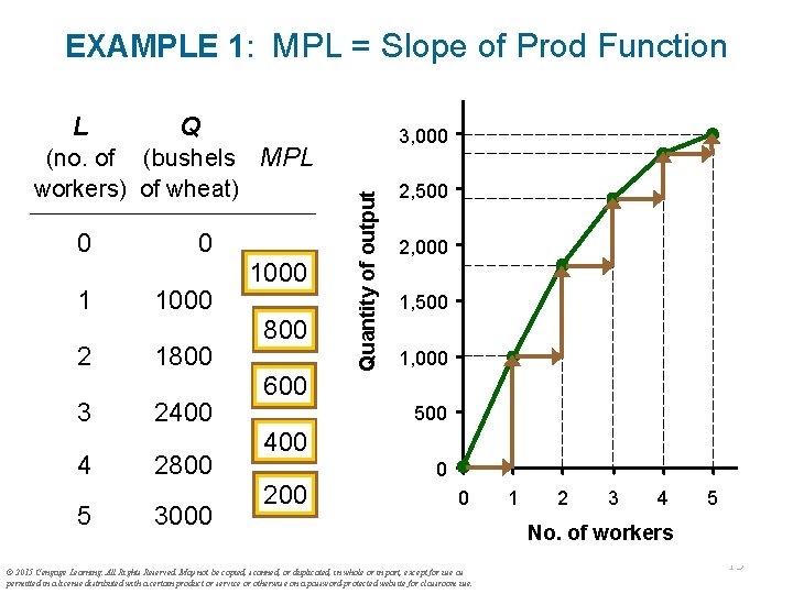
EXAMPLE 1: Farmer Slavko’s Production Function Q (no. of (bushels workers) of wheat) 3, 000 Quantity of output L 2, 500 0 0 1 1000 2 1800 3 2400 500 4 2800 0 5 3000 2, 000 1, 500 1, 000 0 © 2015 Cengage Learning. All Rights Reserved. May not be copied, scanned, or duplicated, in whole or in part, except for use as permitted in a license distributed with a certain product or service or otherwise on a password-protected website for classroom use. 1 2 3 4 5 No. of workers 10

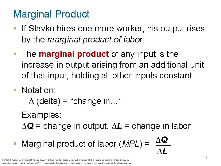
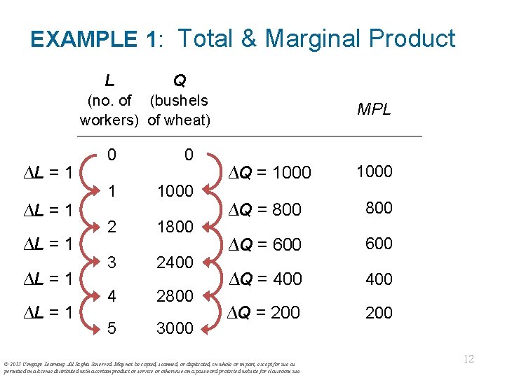
Marginal Product § If Slavko hires one more worker, his output rises by the marginal product of labor. § The marginal product of any input is the increase in output arising from an additional unit of that input, holding all other inputs constant. § Notation: ∆ (delta) = “change in…” Examples: ∆Q = change in output, ∆L = change in labor § Marginal product of labor (MPL) = ∆Q ∆L © 2015 Cengage Learning. All Rights Reserved. May not be copied, scanned, or duplicated, in whole or in part, except for use as permitted in a license distributed with a certain product or service or otherwise on a password-protected website for classroom use. 11

EXAMPLE 1: Total & Marginal Product L Q (no. of (bushels workers) of wheat) ∆L = 1 ∆L = 1 0 0 1 1000 2 1800 3 2400 4 2800 5 3000 MPL ∆Q = 1000 ∆Q = 800 ∆Q = 600 ∆Q = 400 ∆Q = 200 © 2015 Cengage Learning. All Rights Reserved. May not be copied, scanned, or duplicated, in whole or in part, except for use as permitted in a license distributed with a certain product or service or otherwise on a password-protected website for classroom use. 12

EXAMPLE 1: MPL = Slope of Prod Function Q (no. of (bushels MPL workers) of wheat) 0 1 2 3 4 5 0 1000 1800 2400 2800 3000 1000 800 600 400 200 3, 000 MPL Quantity of output L equals the slope of the 2, 500 production function. 2, 000 Notice that MPL diminishes 1, 500 as L increases. 1, 000 This explains why 500 production the function gets flatter 0 as L 0 increases. 1 2 3 © 2015 Cengage Learning. All Rights Reserved. May not be copied, scanned, or duplicated, in whole or in part, except for use as permitted in a license distributed with a certain product or service or otherwise on a password-protected website for classroom use. 4 5 No. of workers 13

Why MPL Is Important § Recall one of the Ten Principles: Rational people think at the margin. § When Farmer Slavko hires an extra worker, § his costs rise by the wage he pays the worker § his output rises by MPL § Comparing them helps Slavko decide whether he should hire the worker. © 2015 Cengage Learning. All Rights Reserved. May not be copied, scanned, or duplicated, in whole or in part, except for use as permitted in a license distributed with a certain product or service or otherwise on a password-protected website for classroom use.

Why MPL Diminishes § Farmer Slavko’s output rises by a smaller and smaller amount for each additional worker. Why? § As he adds workers, the average worker has less land to work with and will be less productive. § In general, MPL diminishes as L rises whether the fixed input is land or capital (equipment, machines, etc. ). § Diminishing marginal product: The marginal product of an input declines as the quantity of the input increases (other things equal). © 2015 Cengage Learning. All Rights Reserved. May not be copied, scanned, or duplicated, in whole or in part, except for use as permitted in a license distributed with a certain product or service or otherwise on a password-protected website for classroom use.

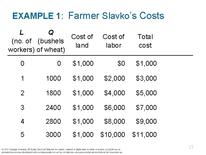
EXAMPLE 1: Farmer Slavko’s Costs § Farmer must pay $1000 per month for the land, regardless of how much wheat he grows. § The market wage for a farm worker is $2000 per month. § So Slavko’s costs are related to how much wheat he produces…. © 2015 Cengage Learning. All Rights Reserved. May not be copied, scanned, or duplicated, in whole or in part, except for use as permitted in a license distributed with a certain product or service or otherwise on a password-protected website for classroom use. 16

EXAMPLE 1: Farmer Slavko’s Costs L Q Cost of (no. of (bushels land workers) of wheat) Cost of labor Total cost 0 0 $1, 000 $0 $1, 000 1 1000 $1, 000 $2, 000 $3, 000 2 1800 $1, 000 $4, 000 $5, 000 3 2400 $1, 000 $6, 000 $7, 000 4 2800 $1, 000 $8, 000 $9, 000 5 3000 $1, 000 $10, 000 $11, 000 © 2015 Cengage Learning. All Rights Reserved. May not be copied, scanned, or duplicated, in whole or in part, except for use as permitted in a license distributed with a certain product or service or otherwise on a password-protected website for classroom use. 17

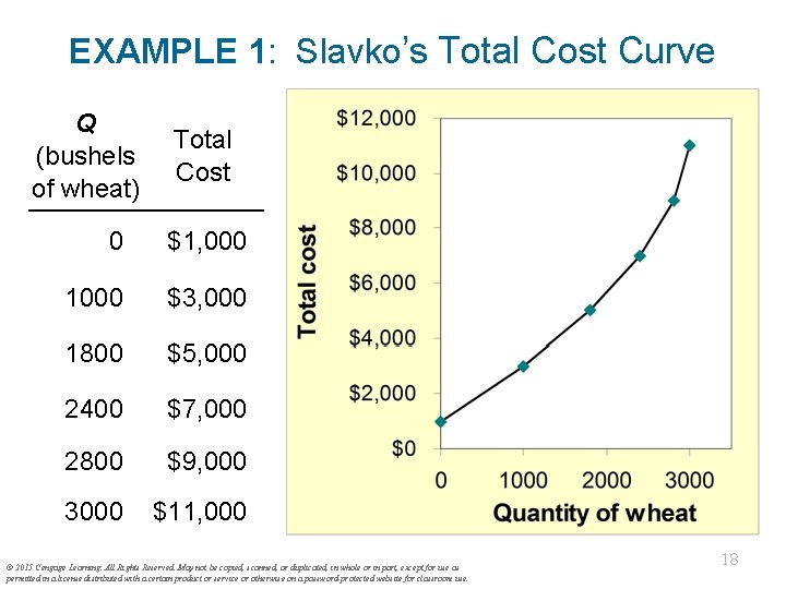
EXAMPLE 1: Slavko’s Total Cost Curve Q (bushels of wheat) Total Cost 0 $1, 000 1000 $3, 000 1800 $5, 000 2400 $7, 000 2800 $9, 000 3000 $11, 000 © 2015 Cengage Learning. All Rights Reserved. May not be copied, scanned, or duplicated, in whole or in part, except for use as permitted in a license distributed with a certain product or service or otherwise on a password-protected website for classroom use. 18

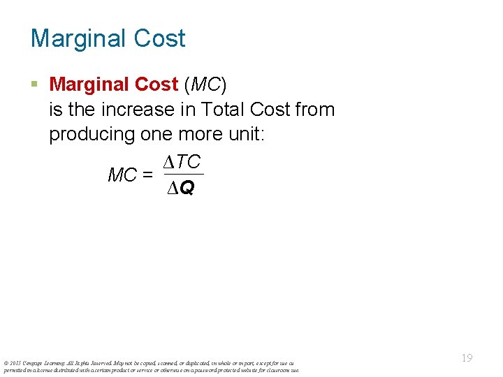
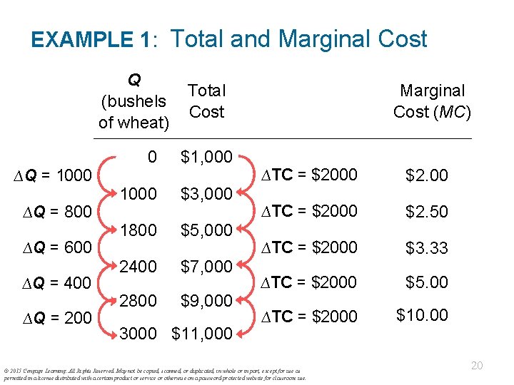
Marginal Cost § Marginal Cost (MC) is the increase in Total Cost from producing one more unit: ∆TC MC = ∆Q © 2015 Cengage Learning. All Rights Reserved. May not be copied, scanned, or duplicated, in whole or in part, except for use as permitted in a license distributed with a certain product or service or otherwise on a password-protected website for classroom use. 19

EXAMPLE 1: Total and Marginal Cost Q (bushels of wheat) ∆Q = 1000 ∆Q = 800 ∆Q = 600 ∆Q = 400 ∆Q = 200 Marginal Cost (MC) Total Cost 0 $1, 000 1000 $3, 000 1800 $5, 000 2400 $7, 000 2800 $9, 000 3000 $11, 000 ∆TC = $2000 $2. 50 ∆TC = $2000 $3. 33 ∆TC = $2000 $5. 00 ∆TC = $2000 $10. 00 © 2015 Cengage Learning. All Rights Reserved. May not be copied, scanned, or duplicated, in whole or in part, except for use as permitted in a license distributed with a certain product or service or otherwise on a password-protected website for classroom use. 20

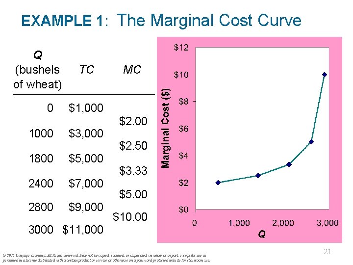
EXAMPLE 1: The Marginal Cost Curve Q (bushels of wheat) 0 TC MC $1, 000 1000 $3, 000 1800 $5, 000 2400 $7, 000 2800 $9, 000 3000 $11, 000 MC usually rises as Q rises, as in this example. $2. 00 $2. 50 $3. 33 $5. 00 $10. 00 © 2015 Cengage Learning. All Rights Reserved. May not be copied, scanned, or duplicated, in whole or in part, except for use as permitted in a license distributed with a certain product or service or otherwise on a password-protected website for classroom use. 21

Why MC Is Important § Farmer Slavko is rational and wants to maximize his profit. To increase profit, should he produce more or less wheat? § To find the answer, he needs to “think at the margin. ” § If the cost of an additional wheat (MC) is less than the revenue he would get from selling it, then Alejandro’s profits rise if he produces more. © 2015 Cengage Learning. All Rights Reserved. May not be copied, scanned, or duplicated, in whole or in part, except for use as permitted in a license distributed with a certain product or service or otherwise on a password-protected website for classroom use.

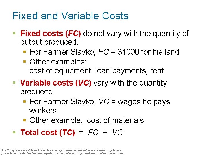
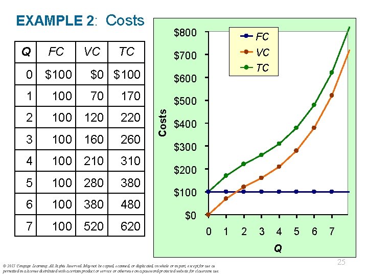
Fixed and Variable Costs § Fixed costs (FC) do not vary with the quantity of output produced. § For Farmer Slavko, FC = $1000 for his land § Other examples: cost of equipment, loan payments, rent § Variable costs (VC) vary with the quantity produced. § For Farmer Slavko, VC = wages he pays workers § Other example: cost of materials § Total cost (TC) = FC + VC © 2015 Cengage Learning. All Rights Reserved. May not be copied, scanned, or duplicated, in whole or in part, except for use as permitted in a license distributed with a certain product or service or otherwise on a password-protected website for classroom use.

EXAMPLE 2 § Our second example is more general, applies to any type of firm producing any good with any types of inputs. © 2015 Cengage Learning. All Rights Reserved. May not be copied, scanned, or duplicated, in whole or in part, except for use as permitted in a license distributed with a certain product or service or otherwise on a password-protected website for classroom use.

EXAMPLE 2: Costs Q FC VC TC $800 FC $700 VC $0 $100 $600 1 100 70 170 $500 2 100 120 220 3 100 160 260 4 100 210 310 5 100 280 380 6 100 380 480 7 100 520 620 Costs 0 $100 TC $400 $300 $200 $100 $0 0 1 2 3 4 5 6 7 Q © 2015 Cengage Learning. All Rights Reserved. May not be copied, scanned, or duplicated, in whole or in part, except for use as permitted in a license distributed with a certain product or service or otherwise on a password-protected website for classroom use. 25

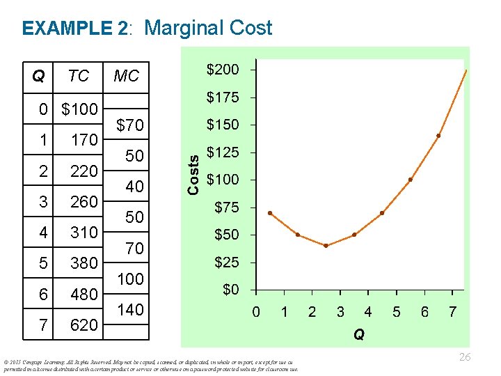
EXAMPLE 2: Marginal Cost Q TC 0 $100 1 170 2 220 3 260 4 310 5 380 6 480 7 620 MC $70 50 40 50 70 100 140 Recall, Marginal Cost (MC) is the change in total cost from producing one more unit: ∆TC MC = ∆Q Usually, MC rises as Q rises, due to diminishing marginal product. Sometimes (as here), MC falls before rising. (In other examples, MC may be constant. ) © 2015 Cengage Learning. All Rights Reserved. May not be copied, scanned, or duplicated, in whole or in part, except for use as permitted in a license distributed with a certain product or service or otherwise on a password-protected website for classroom use. 26

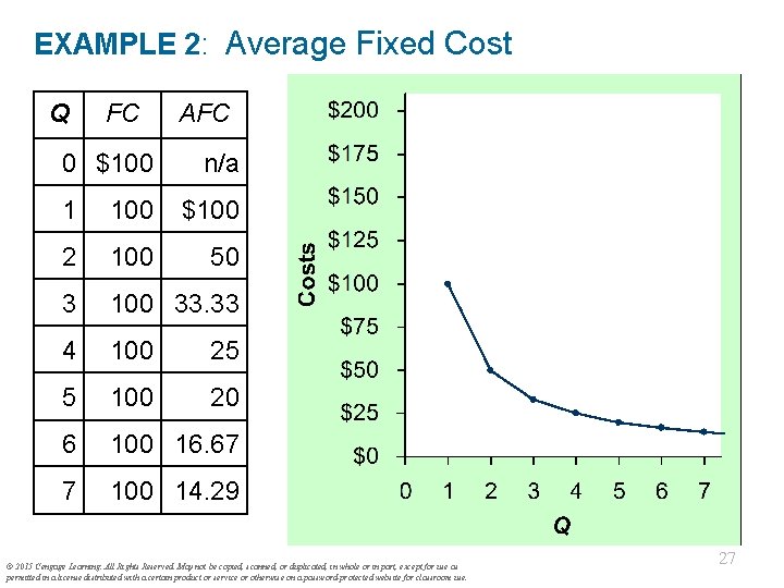
EXAMPLE 2: Average Fixed Cost Q FC 0 $100 AFC n/a 1 100 $100 2 100 50 3 100 33. 33 4 100 25 5 100 20 6 100 16. 67 7 100 14. 29 Average fixed cost (AFC) is fixed cost divided by the quantity of output: AFC = FC/Q Notice that AFC falls as Q rises: The firm is spreading its fixed costs over a larger and larger number of units. © 2015 Cengage Learning. All Rights Reserved. May not be copied, scanned, or duplicated, in whole or in part, except for use as permitted in a license distributed with a certain product or service or otherwise on a password-protected website for classroom use. 27

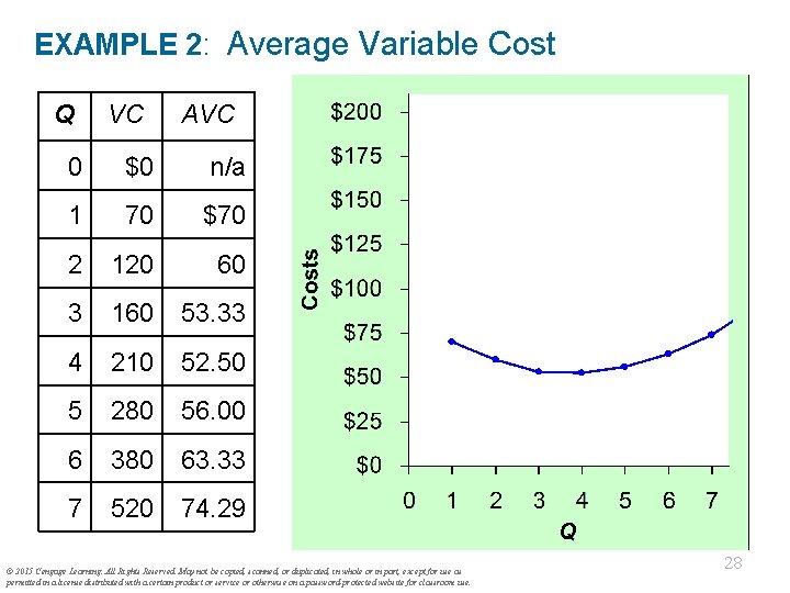
EXAMPLE 2: Average Variable Cost Q VC AVC 0 $0 n/a 1 70 $70 2 120 60 3 160 53. 33 4 210 52. 50 5 280 56. 00 6 380 63. 33 7 520 74. 29 Average variable cost (AVC) is variable cost divided by the quantity of output: AVC = VC/Q As Q rises, AVC may fall initially. In most cases, AVC will eventually rise as output rises. © 2015 Cengage Learning. All Rights Reserved. May not be copied, scanned, or duplicated, in whole or in part, except for use as permitted in a license distributed with a certain product or service or otherwise on a password-protected website for classroom use. 28

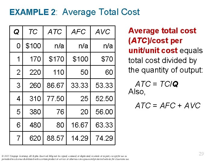
EXAMPLE 2: Average Total Cost Q TC 0 $100 ATC AFC AVC n/a n/a 1 170 $100 $70 2 220 110 50 60 3 260 86. 67 33. 33 53. 33 4 310 77. 50 25 52. 50 5 380 76 20 56. 00 6 480 80 16. 67 63. 33 7 620 88. 57 14. 29 74. 29 Average total cost (ATC)/cost per unit/unit cost equals total cost divided by the quantity of output: ATC = TC/Q Also, © 2015 Cengage Learning. All Rights Reserved. May not be copied, scanned, or duplicated, in whole or in part, except for use as permitted in a license distributed with a certain product or service or otherwise on a password-protected website for classroom use. ATC = AFC + AVC 29

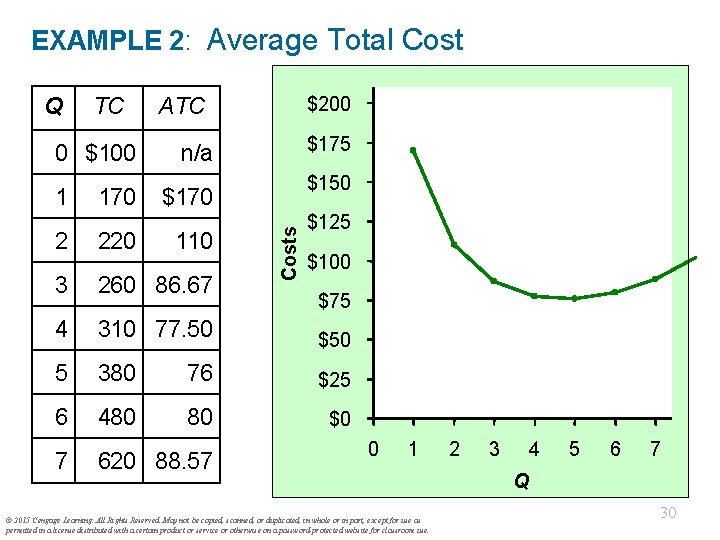
EXAMPLE 2: Average Total Cost TC 0 $100 1 170 ATC $200 Usually, as in this example, $175 the ATC curve is U-shaped. n/a $150 $170 110 Costs Q $125 2 220 3 260 86. 67 4 310 77. 50 $50 5 380 76 $25 6 480 80 $0 7 620 88. 57 $100 $75 0 1 © 2015 Cengage Learning. All Rights Reserved. May not be copied, scanned, or duplicated, in whole or in part, except for use as permitted in a license distributed with a certain product or service or otherwise on a password-protected website for classroom use. 2 3 4 5 6 7 Q 30

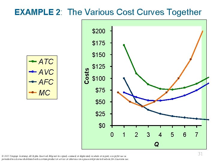
EXAMPLE 2: The Various Cost Curves Together $200 $175 Costs ATC AVC AFC MC $150 $125 $100 $75 $50 $25 $0 0 1 2 3 4 5 6 7 Q © 2015 Cengage Learning. All Rights Reserved. May not be copied, scanned, or duplicated, in whole or in part, except for use as permitted in a license distributed with a certain product or service or otherwise on a password-protected website for classroom use. 31

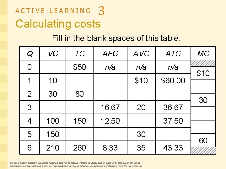
ACTIVE LEARNING 3 Calculating costs Fill in the blank spaces of this table. Q VC 0 1 10 2 30 TC AFC AVC ATC $50 n/a n/a $10 $60. 00 80 3 16. 67 4 100 5 150 6 210 150 20 12. 50 36. 67 8. 33 $10 30 37. 50 30 260 MC 35 © 2015 Cengage Learning. All Rights Reserved. May not be copied, scanned, or duplicated, in whole or in part, except for use as permitted in a license distributed with a certain product or service or otherwise on a password-protected website for classroom use. 43. 33 60

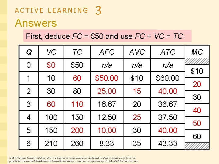
ACTIVE LEARNING Answers 3 Use AFC == FC/Q ATC AVC TC/Q VC/Q MC and First, relationship deduce FC between = $50 and use FCTC + VC = TC. Q VC TC AFC AVC ATC 0 $0 $50 n/a n/a 1 10 60 $50. 00 $10 $60. 00 2 30 80 25. 00 15 40. 00 3 60 110 16. 67 20 36. 67 4 100 150 12. 50 25 37. 50 5 150 200 10. 00 30 40. 00 6 210 260 8. 33 35 43. 33 © 2015 Cengage Learning. All Rights Reserved. May not be copied, scanned, or duplicated, in whole or in part, except for use as permitted in a license distributed with a certain product or service or otherwise on a password-protected website for classroom use. MC $10 20 30 40 50 60

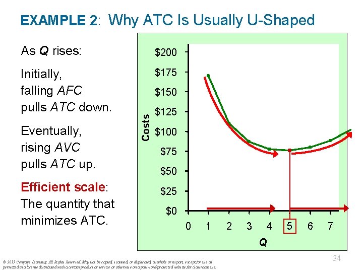
EXAMPLE 2: Why ATC Is Usually U-Shaped As Q rises: $200 Initially, falling AFC pulls ATC down. $175 Efficient scale: The quantity that minimizes ATC. Costs Eventually, rising AVC pulls ATC up. $150 $125 $100 $75 $50 $25 $0 0 1 2 3 4 5 6 7 Q © 2015 Cengage Learning. All Rights Reserved. May not be copied, scanned, or duplicated, in whole or in part, except for use as permitted in a license distributed with a certain product or service or otherwise on a password-protected website for classroom use. 34

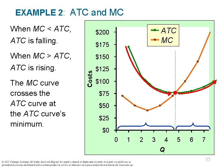
EXAMPLE 2: ATC and MC When MC < ATC, ATC is falling. The MC curve crosses the ATC curve at the ATC curve’s minimum. $175 $150 Costs When MC > ATC, ATC is rising. ATC MC $200 $125 $100 $75 $50 $25 $0 0 1 2 3 4 5 6 7 Q © 2015 Cengage Learning. All Rights Reserved. May not be copied, scanned, or duplicated, in whole or in part, except for use as permitted in a license distributed with a certain product or service or otherwise on a password-protected website for classroom use. 35

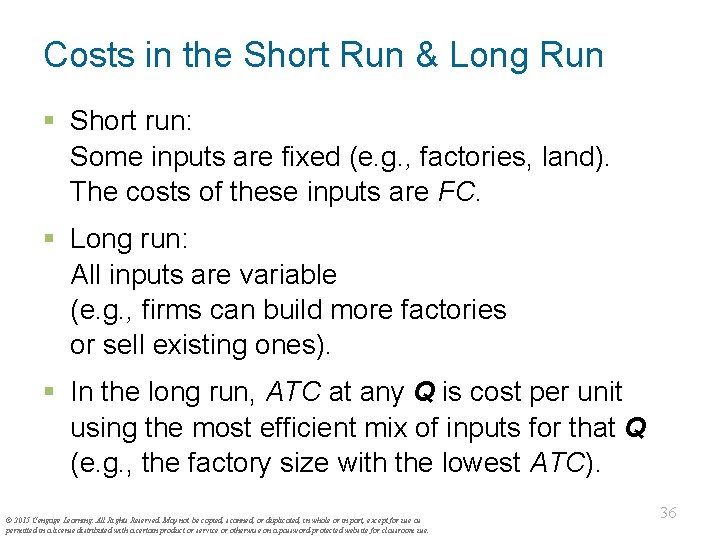
Costs in the Short Run & Long Run § Short run: Some inputs are fixed (e. g. , factories, land). The costs of these inputs are FC. § Long run: All inputs are variable (e. g. , firms can build more factories or sell existing ones). § In the long run, ATC at any Q is cost per unit using the most efficient mix of inputs for that Q (e. g. , the factory size with the lowest ATC). © 2015 Cengage Learning. All Rights Reserved. May not be copied, scanned, or duplicated, in whole or in part, except for use as permitted in a license distributed with a certain product or service or otherwise on a password-protected website for classroom use. 36

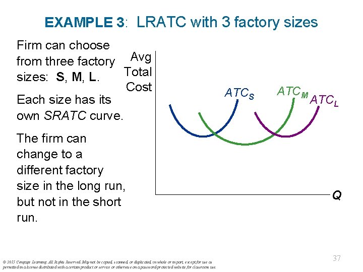
EXAMPLE 3: LRATC with 3 factory sizes Firm can choose from three factory Avg Total sizes: S, M, L. Cost Each size has its own SRATC curve. The firm can change to a different factory size in the long run, but not in the short run. © 2015 Cengage Learning. All Rights Reserved. May not be copied, scanned, or duplicated, in whole or in part, except for use as permitted in a license distributed with a certain product or service or otherwise on a password-protected website for classroom use. ATCS ATCM ATCL Q 37

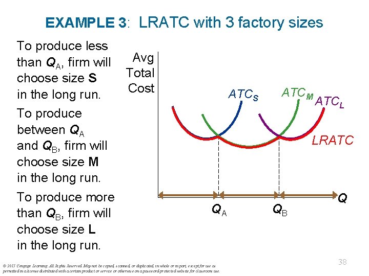
EXAMPLE 3: LRATC with 3 factory sizes To produce less than QA, firm will choose size S in the long run. To produce between QA and QB, firm will choose size M in the long run. To produce more than QB, firm will choose size L in the long run. Avg Total Cost ATCS ATCM ATCL LRATC QA © 2015 Cengage Learning. All Rights Reserved. May not be copied, scanned, or duplicated, in whole or in part, except for use as permitted in a license distributed with a certain product or service or otherwise on a password-protected website for classroom use. QB Q 38

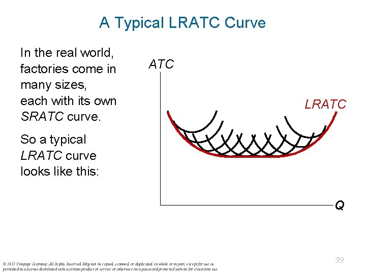
A Typical LRATC Curve In the real world, factories come in many sizes, each with its own SRATC curve. ATC LRATC So a typical LRATC curve looks like this: Q © 2015 Cengage Learning. All Rights Reserved. May not be copied, scanned, or duplicated, in whole or in part, except for use as permitted in a license distributed with a certain product or service or otherwise on a password-protected website for classroom use. 39

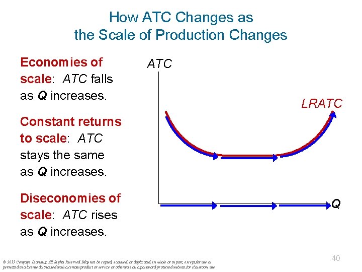
How ATC Changes as the Scale of Production Changes Economies of scale: ATC falls as Q increases. ATC LRATC Constant returns to scale: ATC stays the same as Q increases. Diseconomies of scale: ATC rises as Q increases. © 2015 Cengage Learning. All Rights Reserved. May not be copied, scanned, or duplicated, in whole or in part, except for use as permitted in a license distributed with a certain product or service or otherwise on a password-protected website for classroom use. Q 40

How ATC Changes as the Scale of Production Changes § Economies of scale occur when increasing production allows greater specialization: workers are more efficient when focusing on a narrow task. § More common when Q is low. § Diseconomies of scale are due to coordination problems in large organizations. E. g. , management becomes stretched, can’t control costs. § More common when Q is high. © 2015 Cengage Learning. All Rights Reserved. May not be copied, scanned, or duplicated, in whole or in part, except for use as permitted in a license distributed with a certain product or service or otherwise on a password-protected website for classroom use. 41

CONCLUSION § Costs are critically important to many business decisions including production, pricing, and hiring. § This chapter has introduced the various cost concepts. § The following chapters will show firms use these concepts to maximize profits in various market structures. © 2015 Cengage Learning. All Rights Reserved. May not be copied, scanned, or duplicated, in whole or in part, except for use as permitted in a license distributed with a certain product or service or otherwise on a password-protected website for classroom use. 42

Summary • Implicit costs do not involve a cash outlay, yet are just as important as explicit costs to firms’ decisions. • Accounting profit is revenue minus explicit costs. Economic profit is revenue minus total (explicit + implicit) costs. • The production function shows the relationship between output and inputs. © 2015 Cengage Learning. All Rights Reserved. May not be copied, scanned, or duplicated, in whole or in part, except for use as permitted in a license distributed with a certain product or service or otherwise on a password-protected website for classroom use.

Summary • The marginal product of labor is the increase in output from a one-unit increase in labor, holding other inputs constant. The marginal products of other inputs are defined similarly. • Marginal product usually diminishes as the input increases. Thus, as output rises, the production function becomes flatter and the total cost curve becomes steeper. • Variable costs vary with output; fixed costs do not. © 2015 Cengage Learning. All Rights Reserved. May not be copied, scanned, or duplicated, in whole or in part, except for use as permitted in a license distributed with a certain product or service or otherwise on a password-protected website for classroom use.

Summary • Marginal cost is the increase in total cost from an extra unit of production. The MC curve is usually upward-sloping. • Average variable cost is variable cost divided by output. • Average fixed cost is fixed cost divided by output. AFC always falls as output increases. • Average total cost (sometimes called “cost per unit”) is total cost divided by the quantity of output. The ATC curve is usually U-shaped. © 2015 Cengage Learning. All Rights Reserved. May not be copied, scanned, or duplicated, in whole or in part, except for use as permitted in a license distributed with a certain product or service or otherwise on a password-protected website for classroom use.

Summary • The MC curve intersects the ATC curve at minimum average total cost. When MC < ATC, ATC falls as Q rises. When MC > ATC, ATC rises as Q rises. • In the long run, all costs are variable. • Economies of scale: ATC falls as Q rises. Diseconomies of scale: ATC rises as Q rises. Constant returns to scale: ATC remains constant as Q rises. © 2015 Cengage Learning. All Rights Reserved. May not be copied, scanned, or duplicated, in whole or in part, except for use as permitted in a license distributed with a certain product or service or otherwise on a password-protected website for classroom use.