Week 2 COP 3530 Prefix Averages Method 1

Week 2 COP 3530

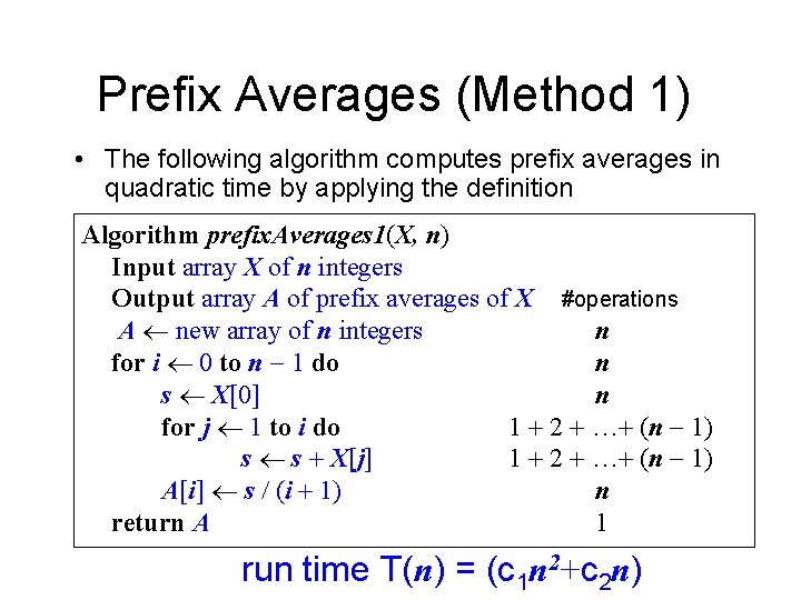
Prefix Averages (Method 1) • The following algorithm computes prefix averages in quadratic time by applying the definition Algorithm prefix. Averages 1(X, n) Input array X of n integers Output array A of prefix averages of X #operations A new array of n integers n for i 0 to n 1 do n s X[0] n for j 1 to i do 1 + 2 + …+ (n 1) s s + X[j] 1 + 2 + …+ (n 1) A[i] s / (i + 1) n return A 1 run time T(n) = (c 1 n 2+c 2 n)

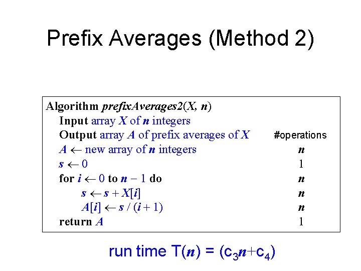
Prefix Averages (Method 2) Algorithm prefix. Averages 2(X, n) Input array X of n integers Output array A of prefix averages of X A new array of n integers s 0 for i 0 to n 1 do s s + X[i] A[i] s / (i + 1) return A #operations run time T(n) = (c 3 n+c 4) n 1 n n n 1

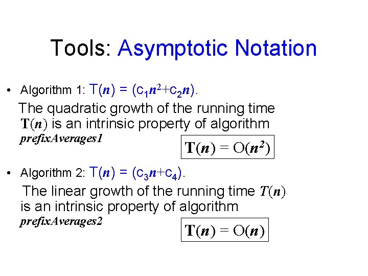
Tools: Asymptotic Notation • Algorithm 1: T(n) = (c 1 n 2+c 2 n). The quadratic growth of the running time T(n) is an intrinsic property of algorithm prefix. Averages 1 T(n) = O(n 2) • Algorithm 2: T(n) = (c 3 n+c 4). The linear growth of the running time T(n) is an intrinsic property of algorithm prefix. Averages 2 T(n) = O(n)

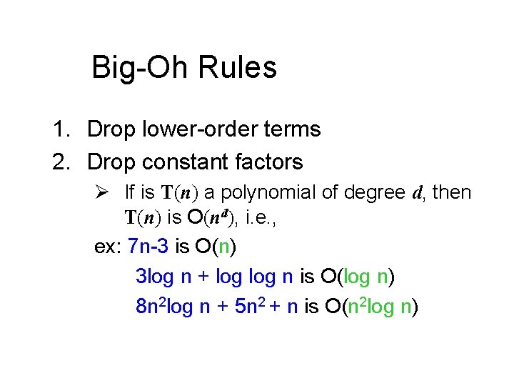
Big-Oh Rules 1. Drop lower-order terms 2. Drop constant factors Ø If is T(n) a polynomial of degree d, then T(n) is O(nd), i. e. , ex: 7 n-3 is O(n) 3 log n + log n is O(log n) 8 n 2 log n + 5 n 2 + n is O(n 2 log n)

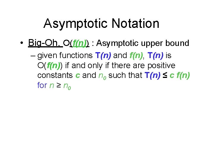
Asymptotic Notation • Big-Oh, O(f(n)) : Asymptotic upper bound – given functions T(n) and f(n), T(n) is O(f(n)) if and only if there are positive constants c and n 0 such that T(n) ≤ c f(n) for n ≥ n 0

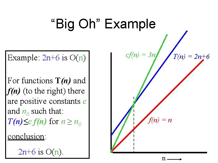
“Big Oh” Example: 2 n+6 is O(n) For functions T(n) and f(n) (to the right) there are positive constants c and n 0 such that: T(n)≤c f(n) for n ≥ n 0 cf(n) = 3 n T(n) = 2 n+6 f(n) = n conclusion: 2 n+6 is O(n). n

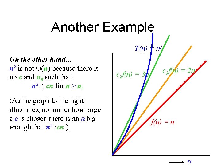
Another Example T(n) = n 2 On the other hand… n 2 is not O(n) because there is no c and n 0 such that: n 2 ≤ cn for n ≥ n 0 (As the graph to the right illustrates, no matter how large a c is chosen there is an n big enough that n 2>cn ). c 2 f(n) = 3 n c 1 f(n) = 2 n f(n) = n n

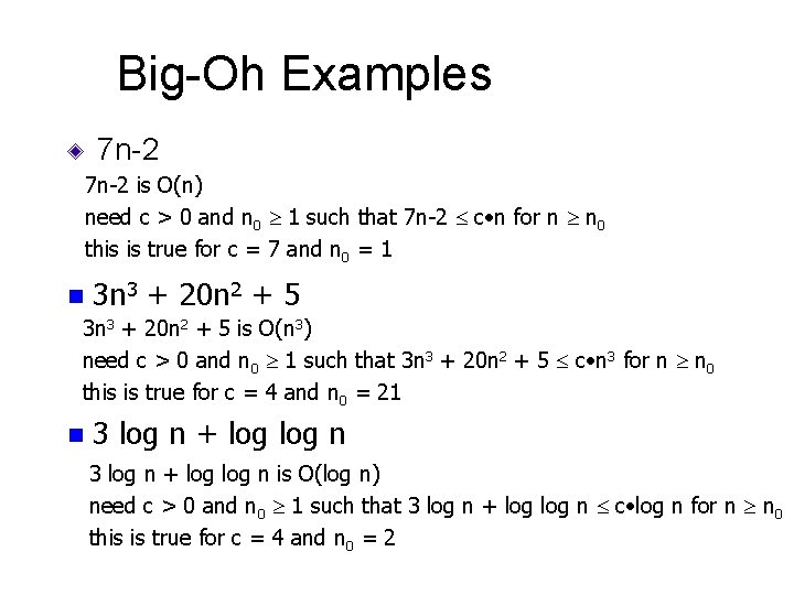
Big-Oh Examples 7 n-2 is O(n) need c > 0 and n 0 1 such that 7 n-2 c • n for n n 0 this is true for c = 7 and n 0 = 1 n 3 n 3 + 20 n 2 + 5 is O(n 3) need c > 0 and n 0 1 such that 3 n 3 + 20 n 2 + 5 c • n 3 for n n 0 this is true for c = 4 and n 0 = 21 n 3 log n + log log n is O(log n) need c > 0 and n 0 1 such that 3 log n + log n c • log n for n n 0 this is true for c = 4 and n 0 = 2

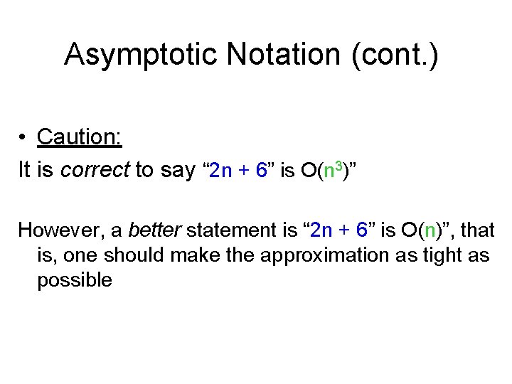
Asymptotic Notation (cont. ) • Caution: It is correct to say “ 2 n + 6” is O(n 3)” However, a better statement is “ 2 n + 6” is O(n)”, that is, one should make the approximation as tight as possible

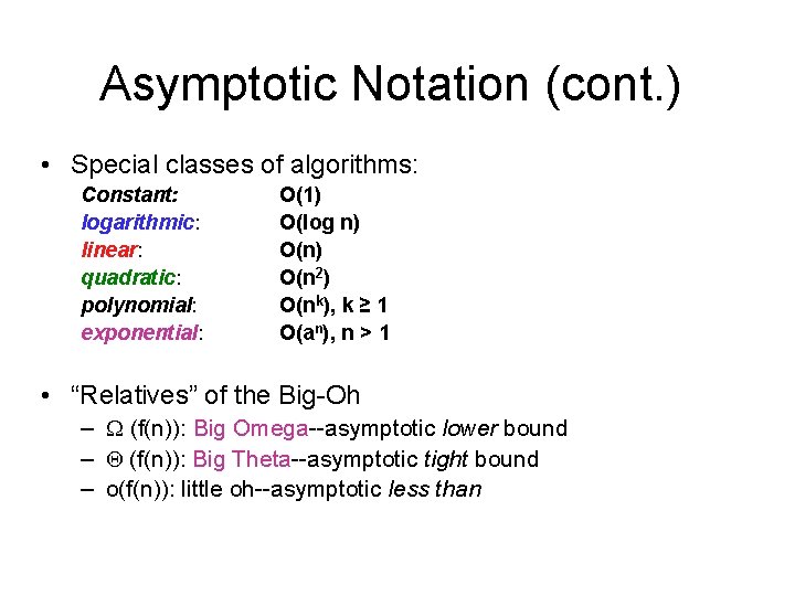
Asymptotic Notation (cont. ) • Special classes of algorithms: Constant: logarithmic: linear: quadratic: polynomial: exponential: O(1) O(log n) O(n 2) O(nk), k ≥ 1 O(an), n > 1 • “Relatives” of the Big-Oh – (f(n)): Big Omega--asymptotic lower bound – (f(n)): Big Theta--asymptotic tight bound – o(f(n)): little oh--asymptotic less than

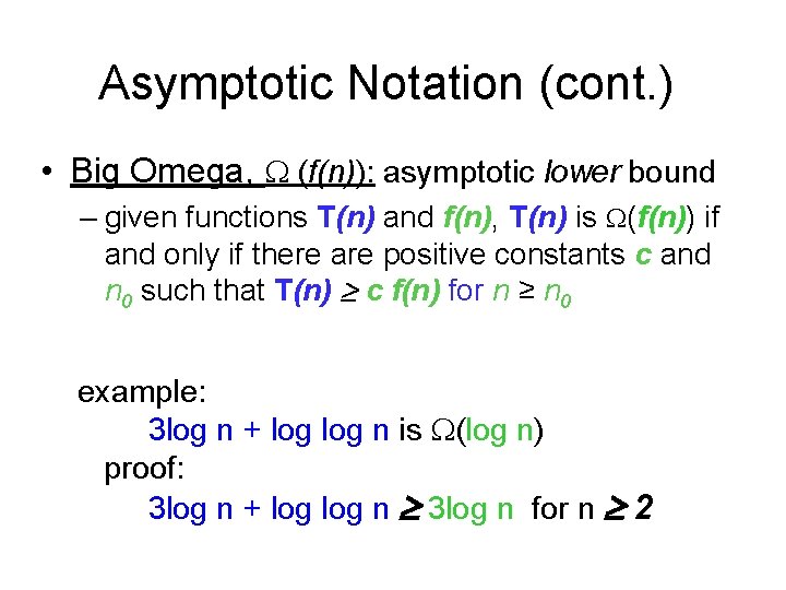
Asymptotic Notation (cont. ) • Big Omega, (f(n)): asymptotic lower bound – given functions T(n) and f(n), T(n) is (f(n)) if and only if there are positive constants c and n 0 such that T(n) c f(n) for n ≥ n 0 example: 3 log n + log n is (log n) proof: 3 log n + log n 3 log n for n 2

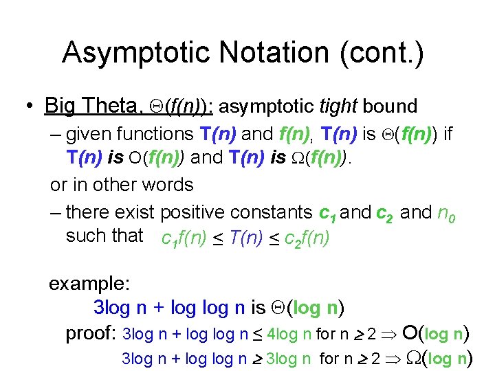
Asymptotic Notation (cont. ) • Big Theta, (f(n)): asymptotic tight bound – given functions T(n) and f(n), T(n) is (f(n)) if T(n) is O(f(n)) and T(n) is (f(n)). or in other words – there exist positive constants c 1 and c 2 and n 0 such that c 1 f(n) ≤ T(n) ≤ c 2 f(n) example: 3 log n + log n is (log n) proof: 3 log n + log n ≤ 4 log n for n 2 O(log n) 3 log n + log n 3 log n for n 2 (log n)

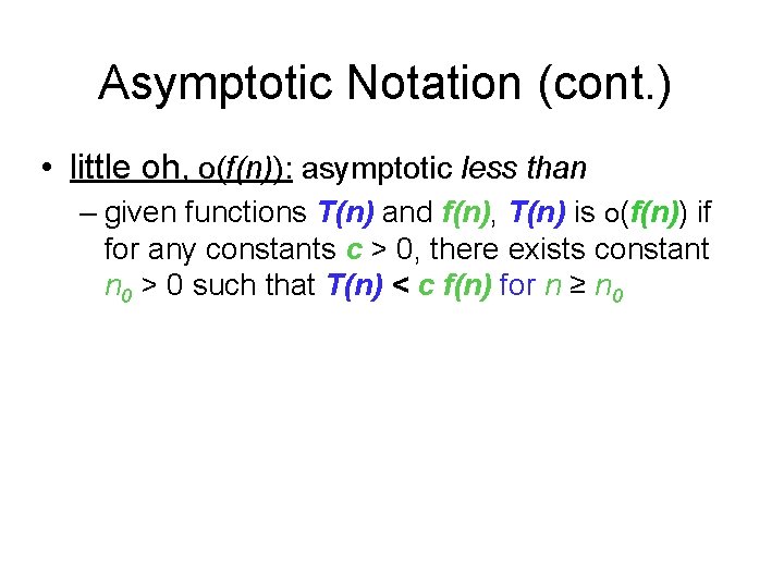
Asymptotic Notation (cont. ) • little oh, o(f(n)): asymptotic less than – given functions T(n) and f(n), T(n) is o(f(n)) if for any constants c > 0, there exists constant n 0 > 0 such that T(n) < c f(n) for n ≥ n 0

Tools: amortization

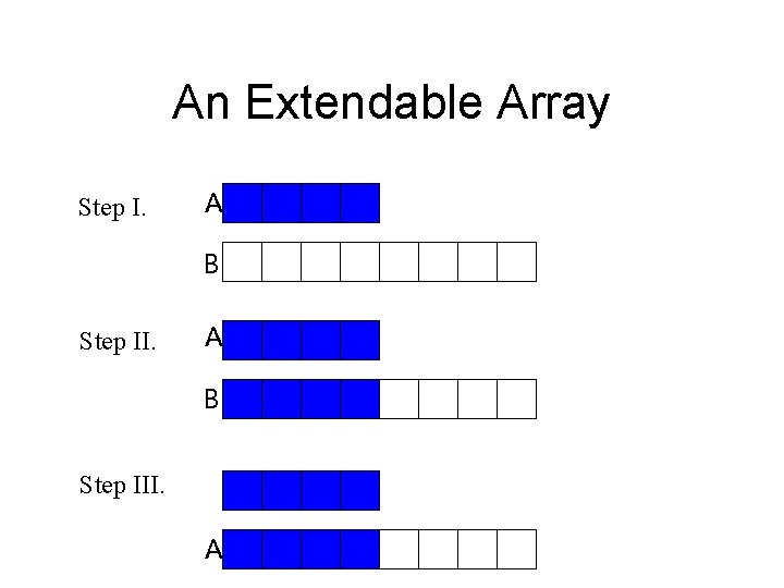
An Extendable Array Step I. A B Step III. A

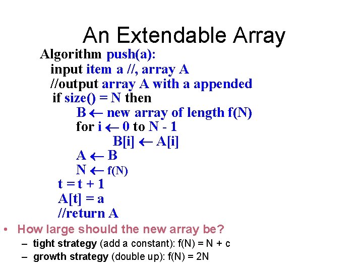
An Extendable Array Algorithm push(a): input item a //, array A //output array A with a appended if size() = N then B new array of length f(N) for i 0 to N - 1 B[i] A[i] A B N f(N) t=t+1 A[t] = a //return A • How large should the new array be? – tight strategy (add a constant): f(N) = N + c – growth strategy (double up): f(N) = 2 N

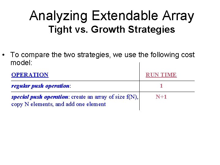
Analyzing Extendable Array Tight vs. Growth Strategies • To compare the two strategies, we use the following cost model: OPERATION regular push operation: special push operation: create an array of size f(N), copy N elements, and add one element RUN TIME 1 N+1

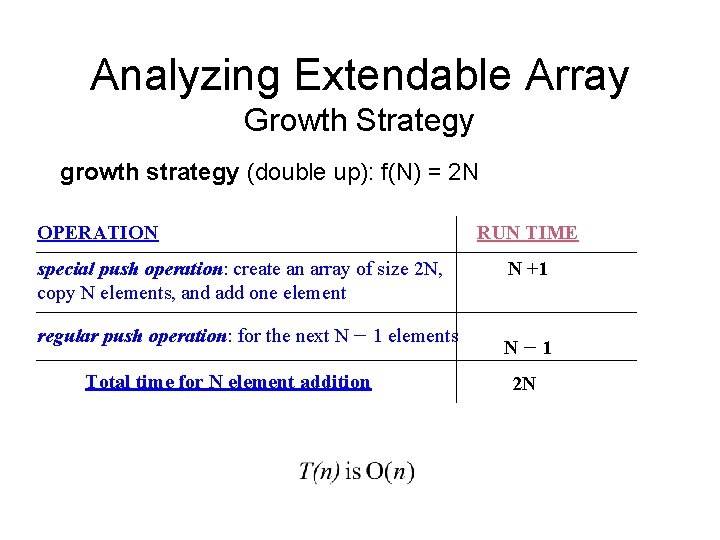
Analyzing Extendable Array Growth Strategy growth strategy (double up): f(N) = 2 N OPERATION special push operation: create an array of size 2 N, copy N elements, and add one element regular push operation: for the next N 1 elements Total time for N element addition RUN TIME N +1 N 1 2 N

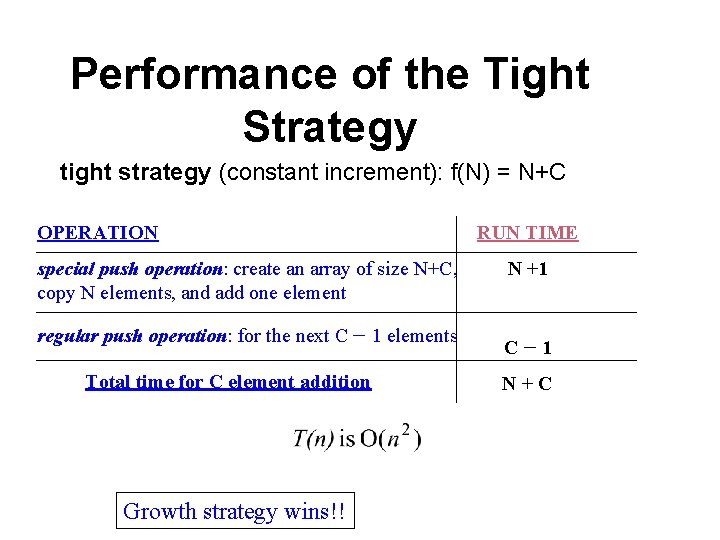
Performance of the Tight Strategy tight strategy (constant increment): f(N) = N+C OPERATION special push operation: create an array of size N+C, copy N elements, and add one element regular push operation: for the next C 1 elements Total time for C element addition Growth strategy wins!! RUN TIME N +1 C 1 N+C

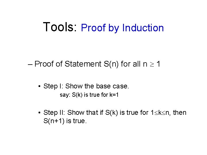
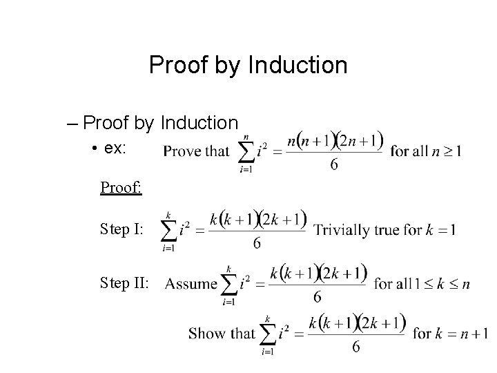
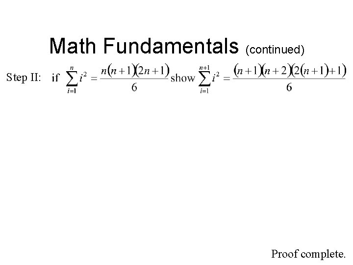
Tools: Proof by Induction – Proof of Statement S(n) for all n 1 • Step I: Show the base case. say: S(k) is true for k=1 • Step II: Show that if S(k) is true for 1 k n, then S(n+1) is true.

Proof by Induction – Proof by Induction • ex: Proof: Step II:

Math Fundamentals (continued) Step II: Proof complete.

Lab Quiz 2

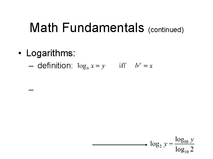
Math Fundamentals (continued) • Logarithms: – definition: –

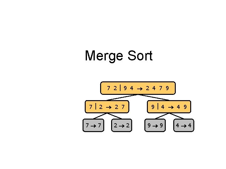
Merge Sort 7 2 9 4 2 4 7 9 7 2 2 7 7 7 2 2 9 4 4 9 9 9 4 4

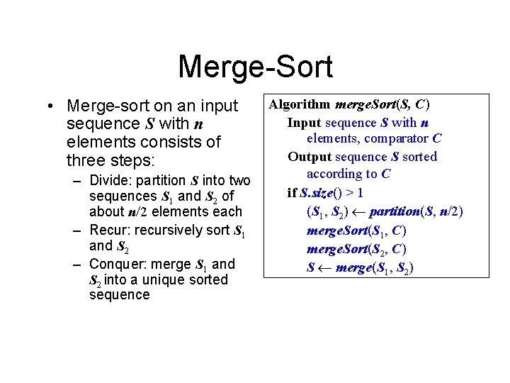
Merge-Sort • Merge-sort on an input sequence S with n elements consists of three steps: – Divide: partition S into two sequences S 1 and S 2 of about n/2 elements each – Recur: recursively sort S 1 and S 2 – Conquer: merge S 1 and S 2 into a unique sorted sequence Algorithm merge. Sort(S, C) Input sequence S with n elements, comparator C Output sequence S sorted according to C if S. size() > 1 (S 1, S 2) partition(S, n/2) merge. Sort(S 1, C) merge. Sort(S 2, C) S merge(S 1, S 2)

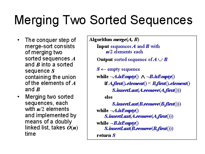
Merging Two Sorted Sequences • The conquer step of merge-sort consists of merging two sorted sequences A and B into a sorted sequence S containing the union of the elements of A and B • Merging two sorted sequences, each with n/2 elements and implemented by means of a doubly linked list, takes O(n) time Algorithm merge(A, B) Input sequences A and B with n/2 elements each Output sorted sequence of A B S empty sequence while A. is. Empty() B. is. Empty() if A. first(). element() < B. first(). element() S. insert. Last(A. remove(A. first())) else S. insert. Last(B. remove(B. first())) while A. is. Empty() S. insert. Last(A. remove(A. first())) while B. is. Empty() S. insert. Last(B. remove(B. first())) return S

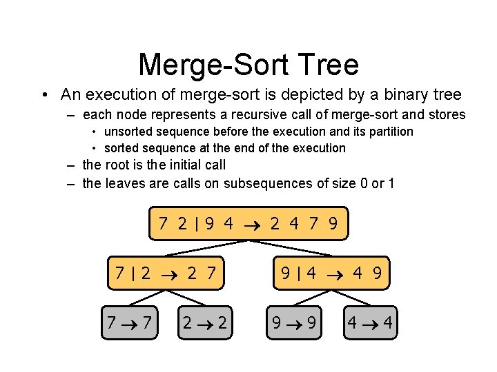
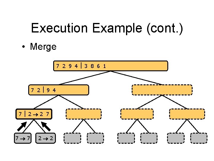
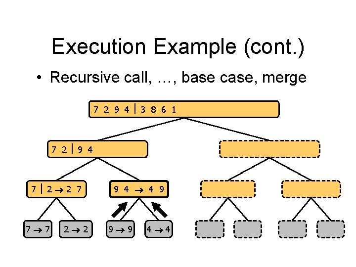
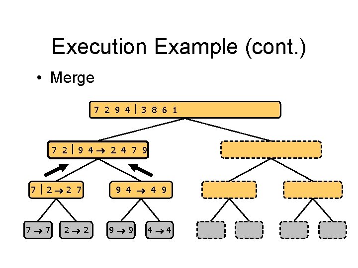
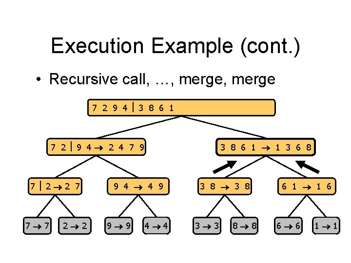
Merge-Sort Tree • An execution of merge-sort is depicted by a binary tree – each node represents a recursive call of merge-sort and stores • unsorted sequence before the execution and its partition • sorted sequence at the end of the execution – the root is the initial call – the leaves are calls on subsequences of size 0 or 1 7 2 7 9 4 2 4 7 9 2 2 7 7 7 2 2 9 4 4 9 9 9 4 4

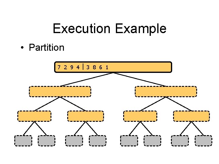
Execution Example • Partition 7 2 9 4 3 8 6 1 1 2 3 4 6 7 8 9 7 2 9 4 2 4 7 9 7 2 2 7 7 7 2 2 3 8 6 1 1 3 8 6 9 4 4 9 9 9 4 4 3 8 3 3 8 8 6 1 1 6 6 6 1 1

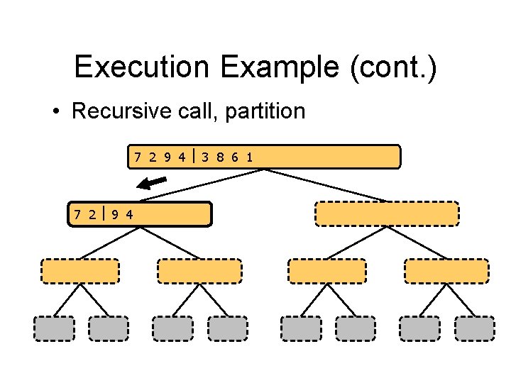
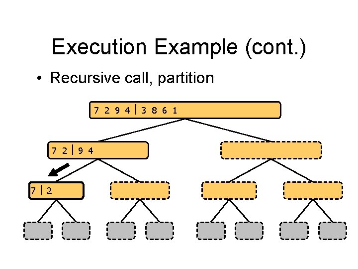
Execution Example (cont. ) • Recursive call, partition 7 2 9 4 3 8 6 1 1 2 3 4 6 7 8 9 7 2 9 4 2 4 7 9 7 2 2 7 7 7 2 2 3 8 6 1 1 3 8 6 9 4 4 9 9 9 4 4 3 8 3 3 8 8 6 1 1 6 6 6 1 1

Execution Example (cont. ) • Recursive call, partition 7 2 9 4 3 8 6 1 1 2 3 4 6 7 8 9 7 2 9 4 2 4 7 9 7 2 2 7 7 7 2 2 3 8 6 1 1 3 8 6 9 4 4 9 9 9 4 4 3 8 3 3 8 8 6 1 1 6 6 6 1 1

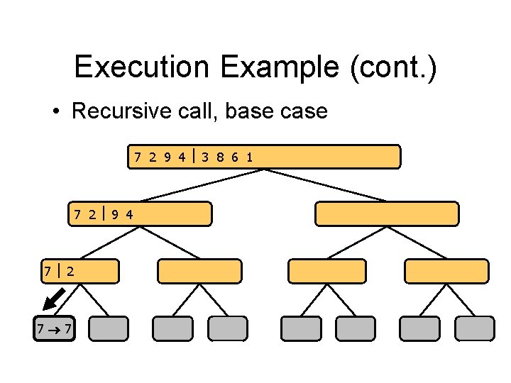
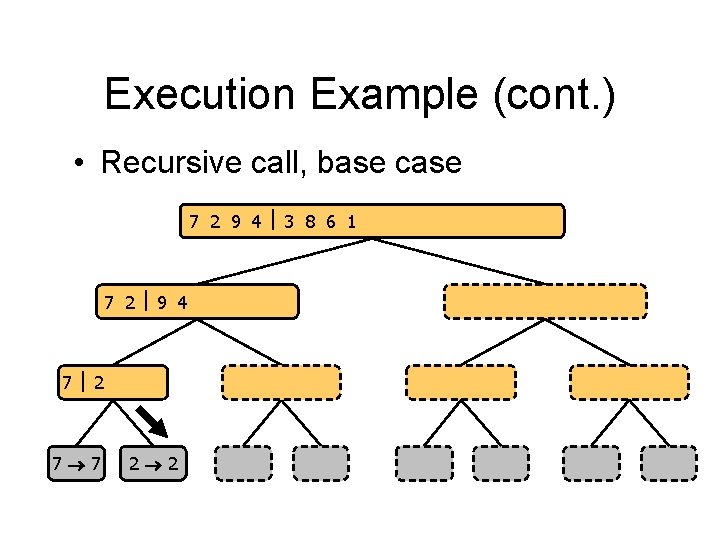
Execution Example (cont. ) • Recursive call, base case 7 2 9 4 3 8 6 1 1 2 3 4 6 7 8 9 7 2 9 4 2 4 7 9 7 2 2 7 7 7 2 2 3 8 6 1 1 3 8 6 9 4 4 9 9 9 4 4 3 8 3 3 8 8 6 1 1 6 6 6 1 1

Execution Example (cont. ) • Recursive call, base case 7 2 9 4 3 8 6 1 1 2 3 4 6 7 8 9 7 2 9 4 2 4 7 9 7 2 2 7 7 7 2 2 3 8 6 1 1 3 8 6 9 4 4 9 9 9 4 4 3 8 3 3 8 8 6 1 1 6 6 6 1 1

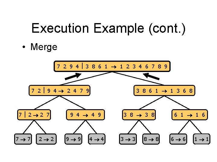
Execution Example (cont. ) • Merge 7 2 9 4 3 8 6 1 1 2 3 4 6 7 8 9 7 2 9 4 2 4 7 9 7 2 2 7 7 7 2 2 3 8 6 1 1 3 8 6 9 4 4 9 9 9 4 4 3 8 3 3 8 8 6 1 1 6 6 6 1 1

Execution Example (cont. ) • Recursive call, …, base case, merge 7 2 9 4 3 8 6 1 1 2 3 4 6 7 8 9 7 2 9 4 2 4 7 9 7 2 2 7 7 7 2 2 3 8 6 1 1 3 8 6 9 4 4 9 9 9 4 4 3 8 3 3 8 8 6 1 1 6 6 6 1 1

Execution Example (cont. ) • Merge 7 2 9 4 3 8 6 1 1 2 3 4 6 7 8 9 7 2 9 4 2 4 7 9 7 2 2 7 7 7 2 2 3 8 6 1 1 3 8 6 9 4 4 9 9 9 4 4 3 8 3 3 8 8 6 1 1 6 6 6 1 1

Execution Example (cont. ) • Recursive call, …, merge 7 2 9 4 3 8 6 1 1 2 3 4 6 7 8 9 7 2 9 4 2 4 7 9 7 2 2 7 7 7 2 2 3 8 6 1 1 3 6 8 9 4 4 9 9 9 4 4 3 8 3 3 8 8 6 1 1 6 6 6 1 1

Execution Example (cont. ) • Merge 7 2 9 4 3 8 6 1 1 2 3 4 6 7 8 9 7 2 9 4 2 4 7 9 7 2 2 7 7 7 2 2 3 8 6 1 1 3 6 8 9 4 4 9 9 9 4 4 3 8 3 3 8 8 6 1 1 6 6 6 1 1

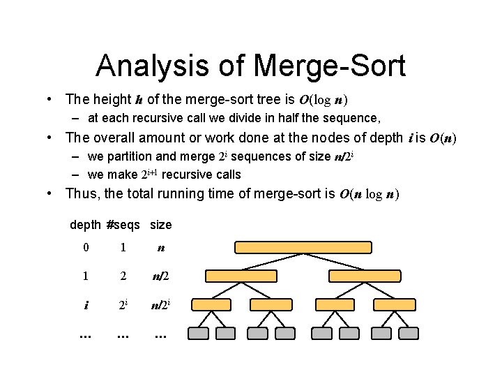
Analysis of Merge-Sort • The height h of the merge-sort tree is O(log n) – at each recursive call we divide in half the sequence, • The overall amount or work done at the nodes of depth i is O(n) – we partition and merge 2 i sequences of size n/2 i – we make 2 i+1 recursive calls • Thus, the total running time of merge-sort is O(n log n) depth #seqs size 0 1 n 1 2 n/2 i 2 i n/2 i … … …

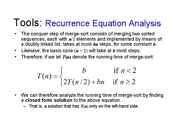
Tools: Recurrence Equation Analysis • The conquer step of merge-sort consists of merging two sorted sequences, each with n/2 elements and implemented by means of a doubly linked list, takes at most bn steps, for some constant b. • Likewise, the basis case (n < 2) will take at b most steps. • Therefore, if we let T(n) denote the running time of merge-sort: • We can therefore analyze the running time of merge-sort by finding a closed form solution to the above equation. – That is, a solution that has T(n) only on the left-hand side.

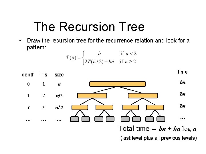
The Recursion Tree • Draw the recursion tree for the recurrence relation and look for a pattern: time depth T’s size 0 1 n bn 1 2 n/2 bn i 2 i n/2 i bn … … Total time = bn + bn log n (last level plus all previous levels)

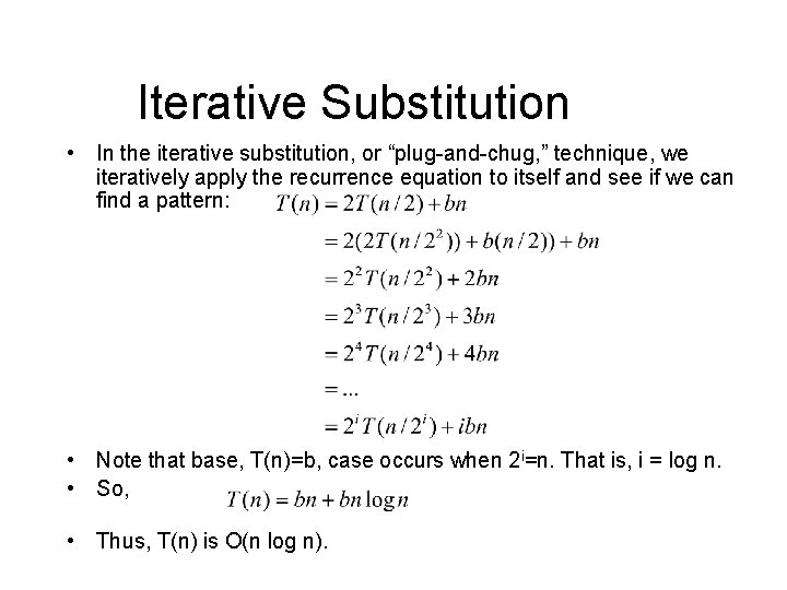
Iterative Substitution • In the iterative substitution, or “plug-and-chug, ” technique, we iteratively apply the recurrence equation to itself and see if we can find a pattern: • Note that base, T(n)=b, case occurs when 2 i=n. That is, i = log n. • So, • Thus, T(n) is O(n log n).

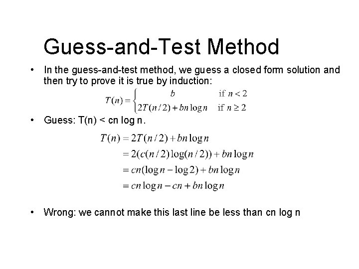
Guess-and-Test Method • In the guess-and-test method, we guess a closed form solution and then try to prove it is true by induction: • Guess: T(n) < cn log n. • Wrong: we cannot make this last line be less than cn log n

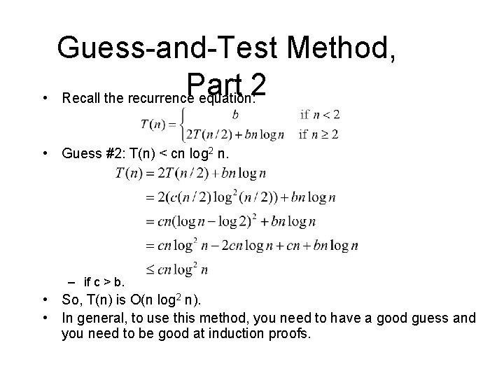
Guess-and-Test Method, Part 2 • Recall the recurrence equation: • Guess #2: T(n) < cn log 2 n. – if c > b. • So, T(n) is O(n log 2 n). • In general, to use this method, you need to have a good guess and you need to be good at induction proofs.

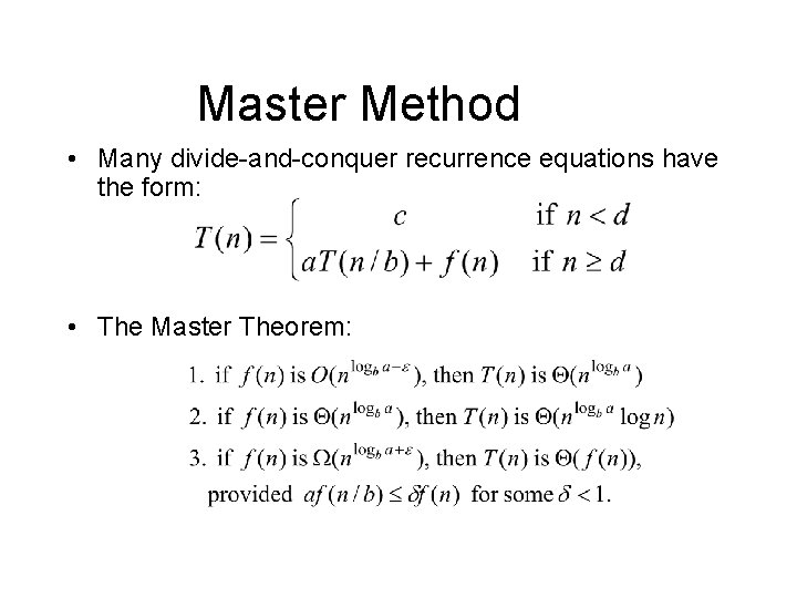
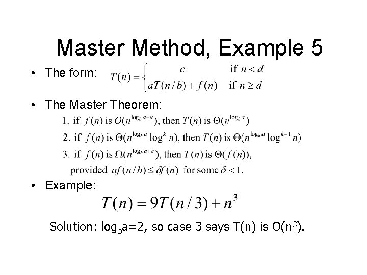
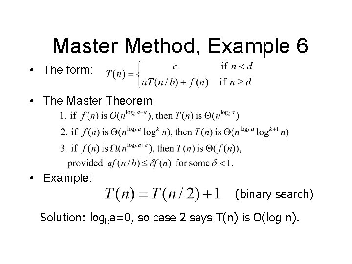
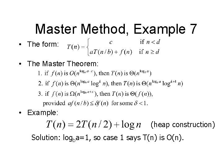
Master Method • Many divide-and-conquer recurrence equations have the form: • The Master Theorem:

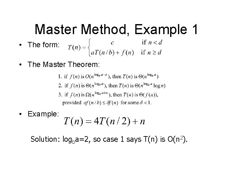
Master Method, Example 1 • The form: • The Master Theorem: • Example: Solution: logba=2, so case 1 says T(n) is O(n 2).

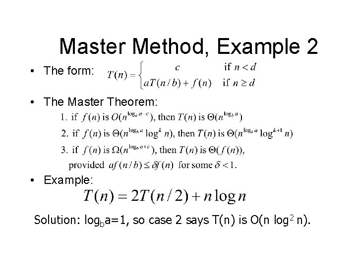
Master Method, Example 2 • The form: • The Master Theorem: • Example: Solution: logba=1, so case 2 says T(n) is O(n log 2 n).

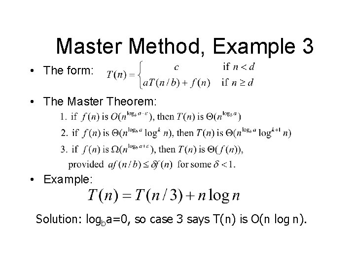
Master Method, Example 3 • The form: • The Master Theorem: • Example: Solution: logba=0, so case 3 says T(n) is O(n log n).

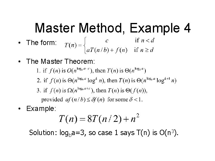
Master Method, Example 4 • The form: • The Master Theorem: • Example: Solution: logba=3, so case 1 says T(n) is O(n 3).

Master Method, Example 5 • The form: • The Master Theorem: • Example: Solution: logba=2, so case 3 says T(n) is O(n 3).

Master Method, Example 6 • The form: • The Master Theorem: • Example: (binary search) Solution: logba=0, so case 2 says T(n) is O(log n).

Master Method, Example 7 • The form: • The Master Theorem: • Example: (heap construction) Solution: logba=1, so case 1 says T(n) is O(n).

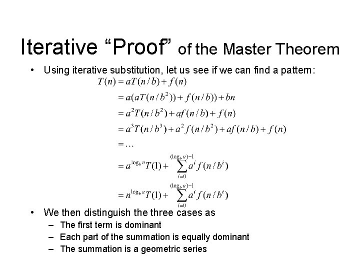
Iterative “Proof” of the Master Theorem • Using iterative substitution, let us see if we can find a pattern: • We then distinguish the three cases as – The first term is dominant – Each part of the summation is equally dominant – The summation is a geometric series