Vector Semantics Introduction Why vector models of meaning

Vector Semantics Introduction

Why vector models of meaning? computing the similarity between words “fast” is similar to “rapid” “tall” is similar to “height” Question answering: Q: “How tall is Mt. Everest? ” Candidate A: “The official height of Mount Everest is 29029 feet” 2

Word similarity for plagiarism detection

Word similarity for historical linguistics: semantic change over time Sagi, Kaufmann Clark 2013 Semantic Broadening 45 40 <1250 35 Middle 1350 -1500 30 Modern 1500 -1710 25 20 15 10 5 0 dog 4 deer hound Kulkarni, Al-Rfou, Perozzi, Skiena 2015

Problems with thesaurus-based meaning • We don’t have a thesaurus for every language • We can’t have a thesaurus for every year • For historical linguistics, we need to compare word meanings in year t to year t+1 • Thesauruses have problems with recall • Many words and phrases are missing • Thesauri work less well for verbs, adjectives

Distributional models of meaning = vector-space models of meaning = vector semantics Intuitions: Zellig Harris (1954): • “oculist and eye-doctor … occur in almost the same environments” • “If A and B have almost identical environments we say that they are synonyms. ” Firth (1957): • “You shall know a word by the company it keeps!” 6

Intuition of distributional word similarity • Nida example: Suppose I asked you what is tesgüino? A bottle of tesgüino is on the table Everybody likes tesgüino Tesgüino makes you drunk We make tesgüino out of corn. • From context words humans can guess tesgüino means • an alcoholic beverage like beer • Intuition for algorithm: • Two words are similar if they have similar word contexts.

Four kinds of vector models Sparse vector representations 1. Mutual-information weighted word co-occurrence matrices Dense vector representations: 2. Singular value decomposition (and Latent Semantic Analysis) 3. Neural-network-inspired models (skip-grams, CBOW) 4. Brown clusters 8

Shared intuition • Model the meaning of a word by “embedding” in a vector space. • The meaning of a word is a vector of numbers • Vector models are also called “embeddings”. • Contrast: word meaning is represented in many computational linguistic applications by a vocabulary index (“word number 545”) • Old philosophy joke: Q: What’s the meaning of life? A: LIFE’ 9

Vector Semantics Words and co-occurrence vectors

Co-occurrence Matrices • We represent how often a word occurs in a document • Term-document matrix • Or how often a word occurs with another 11 • Term-term matrix (or word-word co-occurrence matrix or word-context matrix)

Term-document matrix • Each cell: count of word w in a document d: • Each document is a count vector in ℕv: a column below 12

Similarity in term-document matrices Two documents are similar if their vectors are similar 13

The words in a term-document matrix • Each word is a count vector in ℕD: a row below 14

The words in a term-document matrix • Two words are similar if their vectors are similar 15

The word-word or word-context matrix • 16

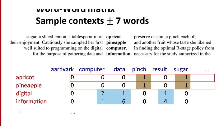
Word-word matrix • 18

2 kinds of co-occurrence between 2 words (Schütze and Pedersen, 1993) • First-order co-occurrence (syntagmatic association): • They are typically nearby each other. • wrote is a first-order associate of book or poem. • Second-order co-occurrence (paradigmatic association): • They have similar neighbors. • wrote is a second- order associate of words like said or remarked. 19

Vector Semantics Positive Pointwise Mutual Information (PPMI)

Problem with raw counts • Raw word frequency is not a great measure of association between words • It’s very skewed • “the” and “of” are very frequent, but maybe not the most discriminative • We’d rather have a measure that asks whether a context word is particularly informative about the target word. • Positive Pointwise Mutual Information (PPMI) 21

Pointwise Mutual Information •

Positive Pointwise Mutual Information •

Computing PPMI on a term-context matrix • Matrix F with W rows (words) and C columns (contexts) • fij is # of times wi occurs in context cj 24

p(w=information, c=data) = 6/19 =. 32 p(w=information) = 11/19 =. 58 p(c=data) = 7/19 =. 37 25

• pmi(information, data) = log 2 (. 32 / (. 37*. 58) ) =. 58 (. 57 using full precision) 26

Weighting PMI • PMI is biased toward infrequent events • Very rare words have very high PMI values • Two solutions: • Give rare words slightly higher probabilities • Use add-one smoothing (which has a similar effect) 27

Weighting PMI: Giving rare context words slightly higher probability • 28

Use Laplace (add-1) smoothing 29

30

PPMI versus add-2 smoothed PPMI 31

Vector Semantics Measuring similarity: the cosine

Measuring similarity • • 33 Given 2 target words v and w We’ll need a way to measure their similarity. Most measure of vectors similarity are based on the: Dot product or inner product from linear algebra • High when two vectors have large values in same dimensions. • Low (in fact 0) for orthogonal vectors with zeros in complementary distribution

Problem with dot product • Dot product is longer if the vector is longer. Vector length: • Vectors are longer if they have higher values in each dimension • That means more frequent words will have higher dot products • That’s bad: we don’t want a similarity metric to be sensitive to 34 word frequency

Solution: cosine • Just divide the dot product by the length of the two vectors! • This turns out to be the cosine of the angle between them! 35

Cosine for computing similarity Dot product Unit vectors vi is the PPMI value for word v in context i wi is the PPMI value for word w in context i. Cos(v, w) is the cosine similarity of v and w Sec. 6. 3

Cosine as a similarity metric • -1: vectors point in opposite directions • +1: vectors point in same directions • 0: vectors are orthogonal • Raw frequency or PPMI are nonnegative, so cosine range 0 -1 37

large data computer apricot 2 0 0 digital 0 1 2 information 1 6 1 Which pair of words is more similar? cosine(apricot, information) = cosine(digital, information) = cosine(apricot, digital) = 38

Visualizing vectors and angles 39 large data apricot 2 0 digital 0 1 information 1 6

Clustering vectors to visualize similarity in co-occurrence matrices 40 Rohde et al. (2006)

Other possible similarity measures

Vector Semantics Measuring similarity: the cosine

Evaluating similarity (the same as for thesaurus-based) • Intrinsic Evaluation: • Correlation between algorithm and human word similarity ratings • Extrinsic (task-based, end-to-end) Evaluation: • Spelling error detection, WSD, essay grading • Taking TOEFL multiple-choice vocabulary tests Levied is closest in meaning to which of these: imposed, believed, requested, correlated

Using syntax to define a word’s context • Zellig Harris (1968) “The meaning of entities, and the meaning of grammatical relations among them, is related to the restriction of combinations of these entities relative to other entities” • Two words are similar if they have similar syntactic contexts Duty and responsibility have similar syntactic distribution: Modified by additional, administrative, assumed, collective, adjectives congressional, constitutional … Objects of verbs assert, assign, assume, attend to, avoid, become, breach. .

Co-occurrence vectors based on syntactic dependencies Dekang Lin, 1998 “Automatic Retrieval and Clustering of Similar Words” • Each dimension: a context word in one of R grammatical relations • Subject-of- “absorb” • Instead of a vector of |V| features, a vector of R|V| • Example: counts for the word cell :

Syntactic dependencies for dimensions • Alternative (Padó and Lapata 2007): Instead of having a |V| x R|V| matrix Have a |V| x |V| matrix But the co-occurrence counts aren’t just counts of words in a window But counts of words that occur in one of R dependencies (subject, object, etc). • So M(“cell”, ”absorb”) = count(subj(cell, absorb)) + count(obj(cell, absorb)) + count(pobj(cell, absorb)), etc. • • 46

PMI applied to dependency relations Hindle, Don. 1990. Noun Classification from Predicate-Argument Structure. ACL Object of “drink” Count PMI it tea 3 2 1. 3 11. 8 anything liquid 3 2 5. 2 10. 5 wine 2 9. 3 tea anything 2 3 11. 8 5. 2 liquid it 2 3 10. 5 1. 3 • “Drink it” more common than “drink wine” • But “wine” is a better “drinkable” thing than “it”

Alternative to PPMI for measuring association • tf-idf (that’s a hyphen not a minus sign) • The combination of two factors • Term frequency (Luhn 1957): frequency of the word (can be logged) • Inverse document frequency (IDF) (Sparck Jones 1972) • N is the total number of documents • dfi = “document frequency of word i” • = # of documents with word I • wij = word i in document j wij=tfij idfi

tf-idf not generally used for word-word similarity • But is by far the most common weighting when we are considering the relationship of words to documents 49

Vector Semantics Dense Vectors

Sparse versus dense vectors • PPMI vectors are • long (length |V|= 20, 000 to 50, 000) • sparse (most elements are zero) • Alternative: learn vectors which are • short (length 200 -1000) • dense (most elements are non-zero) 51

Sparse versus dense vectors • Why dense vectors? • Short vectors may be easier to use as features in machine learning (less weights to tune) • Dense vectors may generalize better than storing explicit counts • They may do better at capturing synonymy: • car and automobile are synonyms; but are represented as distinct dimensions; this fails to capture similarity between a word with car as a neighbor and a word with automobile as a neighbor 52

Three methods for getting short dense vectors • Singular Value Decomposition (SVD) • A special case of this is called LSA – Latent Semantic Analysis • “Neural Language Model”-inspired predictive models • skip-grams and CBOW • Brown clustering 53

Vector Semantics Dense Vectors via SVD

Intuition • Approximate an N-dimensional dataset using fewer dimensions • By first rotating the axes into a new space • In which the highest order dimension captures the most variance in the original dataset • And the next dimension captures the next most variance, etc. • Many such (related) methods: 55 • PCA – principle components analysis • Factor Analysis • SVD

Dimensionality reduction 56

Singular Value Decomposition Any rectangular w x c matrix X equals the product of 3 matrices: W: rows corresponding to original but m columns represents a dimension in a new latent space, such that • M column vectors are orthogonal to each other • Columns are ordered by the amount of variance in the dataset each new dimension accounts for S: diagonal m x m matrix of singular values expressing the importance of each dimension. C: columns corresponding to original but m rows corresponding to 57 singular values

Singular Value Decomposition 58 Landuaer and Dumais 1997

SVD applied to term-document matrix: Latent Semantic Analysis Deerwester et al (1988) • If instead of keeping all m dimensions, we just keep the top k singular values. Let’s say 300. • The result is a least-squares approximation to the original X • But instead of multiplying, we’ll just make use of W. • Each row of W: • A k-dimensional vector • Representing word W 59 / k k / / k

LSA more details • 300 dimensions are commonly used • The cells are commonly weighted by a product of two weights • Local weight: Log term frequency • Global weight: either idf or an entropy measure 60

Let’s return to PPMI word-word matrices • Can we apply to SVD to them? 61

SVD applied to term-term matrix 62 (I’m simplifying here by assuming the matrix has rank |V|)

Truncated SVD on term-term matrix 63

Truncated SVD produces embeddings • Each row of W matrix is a k-dimensional representation of each word w • K might range from 50 to 1000 • Generally we keep the top k dimensions, but some experiments suggest that getting rid of the top 1 dimension or even the top 50 dimensions is helpful (Lapesa and Evert 2014). 64

Embeddings versus sparse vectors • Dense SVD embeddings sometimes work better than sparse PPMI matrices at tasks like word similarity 65 • Denoising: low-order dimensions may represent unimportant information • Truncation may help the models generalize better to unseen data. • Having a smaller number of dimensions may make it easier for classifiers to properly weight the dimensions for the task. • Dense models may do better at capturing higher order cooccurrence.

Vector Semantics Embeddings inspired by neural language models: skip-grams and CBOW

Prediction-based models: An alternative way to get dense vectors • Skip-gram (Mikolov et al. 2013 a) CBOW (Mikolov et al. 2013 b) • Learn embeddings as part of the process of word prediction. • Train a neural network to predict neighboring words • Inspired by neural net language models. • In so doing, learn dense embeddings for the words in the training corpus. • Advantages: 67 • Fast, easy to train (much faster than SVD) • Available online in the word 2 vec package • Including sets of pretrained embeddings!

Skip-grams • Predict each neighboring word • in a context window of 2 C words • from the current word. • So for C=2, we are given word wt and predicting these 4 words: 68

Skip-grams learn 2 embeddings for each w input embedding v, in the input matrix W • Column i of the input matrix W is the 1×d embedding vi for word i in the vocabulary. output embedding v′, in output matrix W’ • Row i of the output matrix W′ is a d × 1 vector embedding v′i for word i in the vocabulary. 69

Setup • Walking through corpus pointing at word w(t), whose index in the vocabulary is j, so we’ll call it wj (1 < j < |V |). • Let’s predict w(t+1) , whose index in the vocabulary is k (1 < k < |V |). Hence our task is to compute P(wk|wj). 70

One-hot vectors • • • 71 A vector of length |V| 1 for the target word and 0 for other words So if “popsicle” is vocabulary word 5 The one-hot vector is [0, 0, 1, 0, 0……. 0]

Skip-gram 72

Skip-gram h = vj o = W’h 73

Skip-gram h = vj o = W’h ok = v’k∙vj 74

Turning outputs into probabilities • ok = v’k∙vj • We use softmax to turn into probabilities 75

Embeddings from W and W’ • Since we have two embeddings, vj and v’j for each word wj • We can either: • Just use vj • Sum them • Concatenate them to make a double-length embedding 76

But wait; how do we learn the embeddings? 77

Relation between skipgrams and PMI! • If we multiply WW’T • We get a |V|x|V| matrix M , each entry mij corresponding to some association between input word i and output word j • Levy and Goldberg (2014 b) show that skip-gram reaches its optimum just when this matrix is a shifted version of PMI: WW′T =MPMI −log k • So skip-gram is implicitly factoring a shifted version of the PMI matrix into the two embedding matrices. 78

CBOW (Continuous Bag of Words) 79

Properties of embeddings • Nearest words to some embeddings (Mikolov et al. 20131) 80

Embeddings capture relational meaning! • 81

Vector Semantics Brown clustering

Brown clustering • An agglomerative clustering algorithm that clusters words based on which words precede or follow them • These word clusters can be turned into a kind of vector • We’ll give a very brief sketch here. 83

Brown clustering algorithm • Each word is initially assigned to its own cluster. • We now consider merging each pair of clusters. Highest quality merge is chosen. • Quality = merges two words that have similar probabilities of preceding and following words • (More technically quality = smallest decrease in the likelihood of the corpus according to a class-based language model) • Clustering proceeds until all words are in one big cluster. 84

Brown Clusters as vectors • By tracing the order in which clusters are merged, the model builds a binary tree from bottom to top. • Each word represented by binary string = path from root to leaf • Each intermediate node is a cluster • Chairman is 0010, “months” = 01, and verbs = 1 85

Brown cluster examples 86

Class-based language model • Suppose each word was in some class ci: 87

Vector Semantics Evaluating similarity

Evaluating similarity • Extrinsic (task-based, end-to-end) Evaluation: • Question Answering • Spell Checking • Essay grading • Intrinsic Evaluation: • Correlation between algorithm and human word similarity ratings • Wordsim 353: 353 noun pairs rated 0 -10. sim(plane, car)=5. 77 • Taking TOEFL multiple-choice vocabulary tests • Levied is closest in meaning to: imposed, believed, requested, correlated

Summary • Distributional (vector) models of meaning • Sparse (PPMI-weighted word-word co-occurrence matrices) • Dense: • Word-word SVD 50 -2000 dimensions • Skip-grams and CBOW • Brown clusters 5 -20 binary dimensions. 90