Vector Data Layout Vector xn P processors Assume

Vector: Data Layout Vector: x[n] P processors Assume n = r * p A[m: n] for(i=m; i<=n) A[i]… Let A[m : s : n] denotes for(i=m; i<=n; i=i+s) A[i] … p r n n/N P*n/N n n Block distribution: id = 0, 1, …, p-1 x[r*id : r*(id+1)-1] id-th processor Cyclic distribution: x[id : p : n-1] id-th processor Block cyclic distribution: x = [x 1, x 2, …, x. N]^T where xj is a subvector of length n/N Assume N = s*p Do a cyclic distribution of xj, j=1, 2…, N block cyclic Block cyclic 1

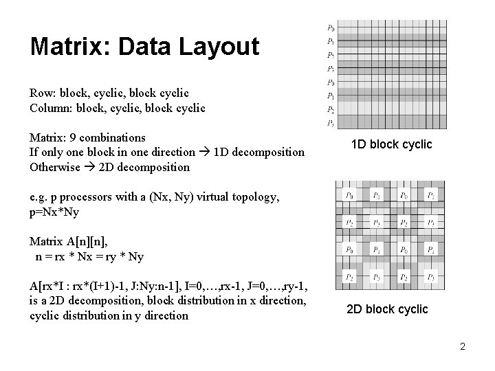
Matrix: Data Layout Row: block, cyclic, block cyclic Column: block, cyclic, block cyclic Matrix: 9 combinations If only one block in one direction 1 D decomposition Otherwise 2 D decomposition 1 D block cyclic e. g. p processors with a (Nx, Ny) virtual topology, p=Nx*Ny Matrix A[n][n], n = rx * Nx = ry * Ny A[rx*I : rx*(I+1)-1, J: Ny: n-1], I=0, …, rx-1, J=0, …, ry-1, is a 2 D decomposition, block distribution in x direction, cyclic distribution in y direction 2 D block cyclic 2

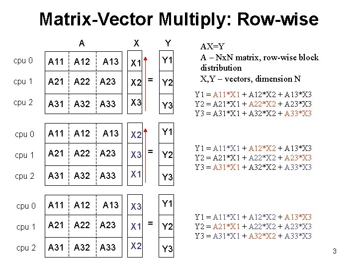
Matrix-Vector Multiply: Row-wise A cpu 0 A 11 A 12 cpu 1 A 22 A 13 A 23 X Y X 1 Y 1 X 2 = Y 2 X 3 Y 3 X 2 Y 1 cpu 2 A 31 A 32 cpu 0 A 11 A 12 cpu 1 A 22 A 23 X 3 = Y 2 cpu 2 A 31 A 32 A 33 X 1 Y 3 cpu 0 A 11 A 12 X 3 Y 1 A 33 A 13 cpu 1 A 22 A 23 X 1 = cpu 2 A 31 A 32 A 33 X 2 Y 3 AX=Y A – Nx. N matrix, row-wise block distribution X, Y – vectors, dimension N Y 1 = A 11*X 1 + A 12*X 2 + A 13*X 3 Y 2 = A 21*X 1 + A 22*X 2 + A 23*X 3 Y 3 = A 31*X 1 + A 32*X 2 + A 33*X 3 3

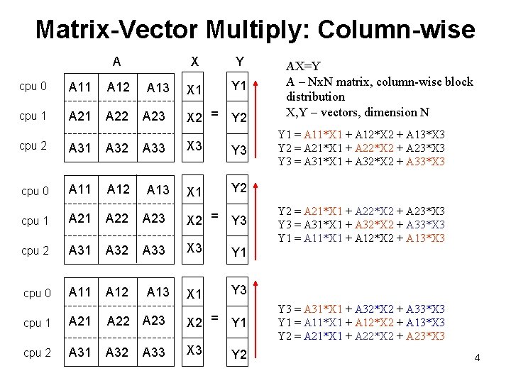
Matrix-Vector Multiply: Column-wise A cpu 0 A 11 A 12 cpu 1 A 22 A 13 A 23 X Y X 1 Y 1 X 2 = Y 2 X 3 Y 3 X 1 Y 2 cpu 2 A 31 A 32 cpu 0 A 11 A 12 cpu 1 A 22 A 23 X 2 = Y 3 cpu 2 A 31 A 32 A 33 X 3 Y 1 cpu 0 A 11 A 12 X 1 Y 3 A 33 A 13 cpu 1 A 22 A 23 X 2 = cpu 2 A 31 A 32 X 3 A 33 Y 1 Y 2 AX=Y A – Nx. N matrix, column-wise block distribution X, Y – vectors, dimension N Y 1 = A 11*X 1 + A 12*X 2 + A 13*X 3 Y 2 = A 21*X 1 + A 22*X 2 + A 23*X 3 Y 3 = A 31*X 1 + A 32*X 2 + A 33*X 3 Y 1 = A 11*X 1 + A 12*X 2 + A 13*X 3 Y 2 = A 21*X 1 + A 22*X 2 + A 23*X 3 4

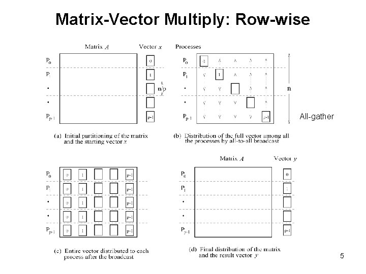
Matrix-Vector Multiply: Row-wise All-gather 5

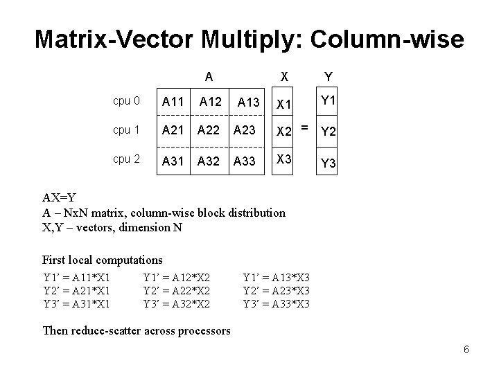
Matrix-Vector Multiply: Column-wise A X Y X 1 Y 1 cpu 0 A 11 A 12 cpu 1 A 22 A 23 X 2 = Y 2 cpu 2 A 31 A 32 A 33 X 3 Y 3 A 13 AX=Y A – Nx. N matrix, column-wise block distribution X, Y – vectors, dimension N First local computations Y 1’ = A 11*X 1 Y 2’ = A 21*X 1 Y 3’ = A 31*X 1 Y 1’ = A 12*X 2 Y 2’ = A 22*X 2 Y 3’ = A 32*X 2 Y 1’ = A 13*X 3 Y 2’ = A 23*X 3 Y 3’ = A 33*X 3 Then reduce-scatter across processors 6

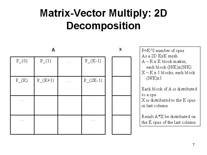
Matrix-Vector Multiply: 2 D Decomposition x A P_{0} P_{1} … P_{K-1} P_{K+1} … P_{2 K-1} Each block of A is distributed to a cpu X is distributed to the K cpus in last column … … P=K^2 number of cpus As a 2 D Kx. K mesh A – K x K block matrix, each block (N/K)x(N/K) X – K x 1 blocks, each block (N/K)x 1 … Result A*X be distributed on the K cpus of the last column 7

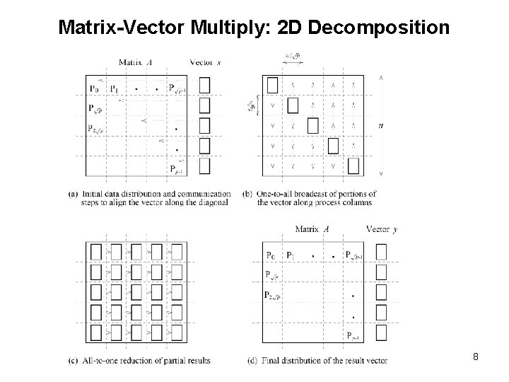
Matrix-Vector Multiply: 2 D Decomposition 8

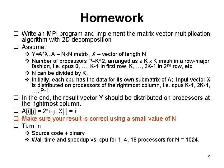
Homework q Write an MPI program and implement the matrix vector multiplication algorithm with 2 D decomposition q Assume: v Y=A*X, A – Nx. N matrix, X – vector of length N v Number of processors P=K^2, arranged as a K x K mesh in a row-major fashion, i. e. cpus 0, …, K-1 in first row, K, …, 2 K-1 in 2 nd row, etc v N can be divided by K. v Initially, each cpu has the data for its own submatrix of A; Input vector X is distributed on processors of the rightmost column, i. e. cpus K-1, 2 K-1, …, P-1 q In the end, the result vector Y should be distributed on processors at the rightmost column. q A[i][j] = 2*i+j, X[i] = i; q Make sure your result is correct using a small value of N q Turn in: v Source code + binary v Wall-time and speedup vs. cpu for 1, 4, 16 processors for N = 1024. 9

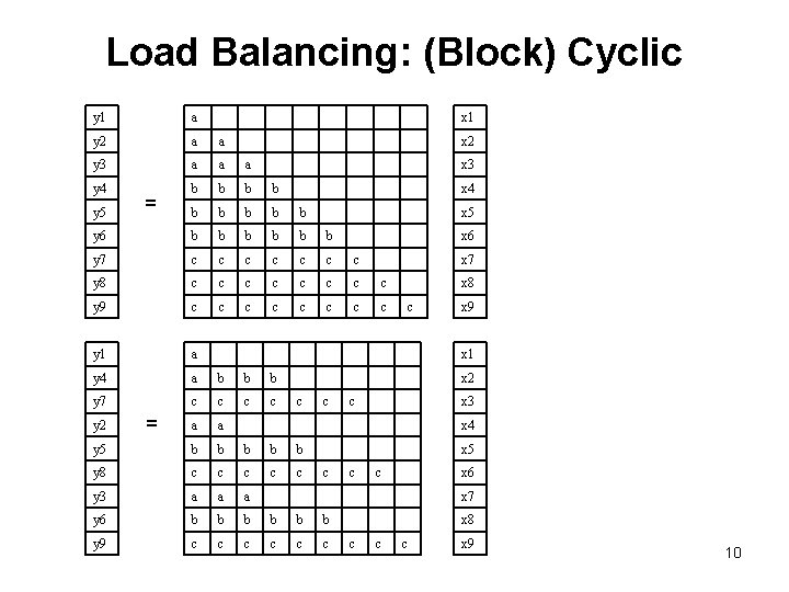
Load Balancing: (Block) Cyclic y 1 a y 2 a a y 3 a a a y 4 b b b b b y 6 b b b y 7 c c c c y 8 c c c c y 9 c c c c y 1 a y 4 a b b b y 7 c c a a y 5 b b b y 8 c c c y 3 a a a y 6 b b b y 9 c c c y 5 y 2 = = x 1 x 2 x 3 x 4 x 5 x 6 x 7 x 8 c x 9 x 1 x 2 c c c x 3 x 4 x 5 c c c x 6 x 7 x 8 c c c x 9 10

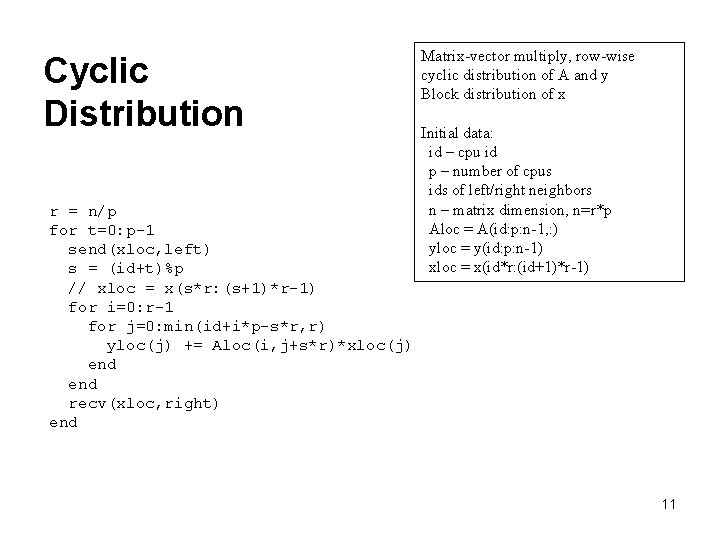
Cyclic Distribution r = n/p for t=0: p-1 send(xloc, left) s = (id+t)%p // xloc = x(s*r: (s+1)*r-1) for i=0: r-1 for j=0: min(id+i*p-s*r, r) yloc(j) += Aloc(i, j+s*r)*xloc(j) end recv(xloc, right) end Matrix-vector multiply, row-wise cyclic distribution of A and y Block distribution of x Initial data: id – cpu id p – number of cpus ids of left/right neighbors n – matrix dimension, n=r*p Aloc = A(id: p: n-1, : ) yloc = y(id: p: n-1) xloc = x(id*r: (id+1)*r-1) 11

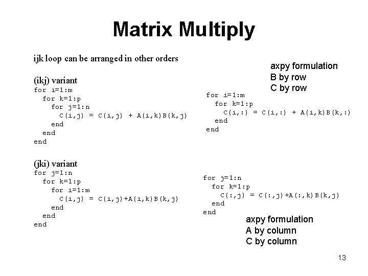
Matrix Multiplication Row: A(i, : ) = [Ai 1, Ai 2, …, Ain] Column: A(: , j) = [A 1 j, A 2 j, …, Anj]^T Submatrix: A(i 1: i 2, j 1: j 2) = [ A(i, j) ], i 1<=i<=i 2, j 1<=j<=j 2 for i=1: m for j=1: n for k=1: p C(i, j) = C(i, j)+A(i, k)*B(k, j) end end for i=1: m for j=1: n C(i, j) = C(i, j)+A(i, : )B(: , j) end A–mxp B–pxn C–mxn C = AB + C (ijk) variant of matrix multiplication Dot product formulation A(i, : ) dot B(: , j) A accessed by row B accessed by column Non-optimal memory access! 12

Matrix Multiply ijk loop can be arranged in other orders (ikj) variant for i=1: m for k=1: p for j=1: n C(i, j) = C(i, j) + A(i, k)B(k, j) end end axpy formulation B by row C by row for i=1: m for k=1: p C(i, : ) = C(i, : ) + A(i, k)B(k, : ) end (jki) variant for j=1: n for k=1: p for i=1: m C(i, j) = C(i, j)+A(i, k)B(k, j) end end for j=1: n for k=1: p C(: , j) = C(: , j)+A(: , k)B(k, j) end axpy formulation A by column C by column 13

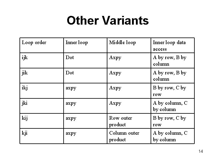
Other Variants Loop order Inner loop Middle loop Inner loop data access ijk Dot Axpy A by row, B by column jik Dot Axpy A by row, B by column ikj axpy Axpy B by row, C by row jki axpy A by column, C by column kij axpy Row outer product B by row, C by row kji axpy Column outer product A by column, C by column 14

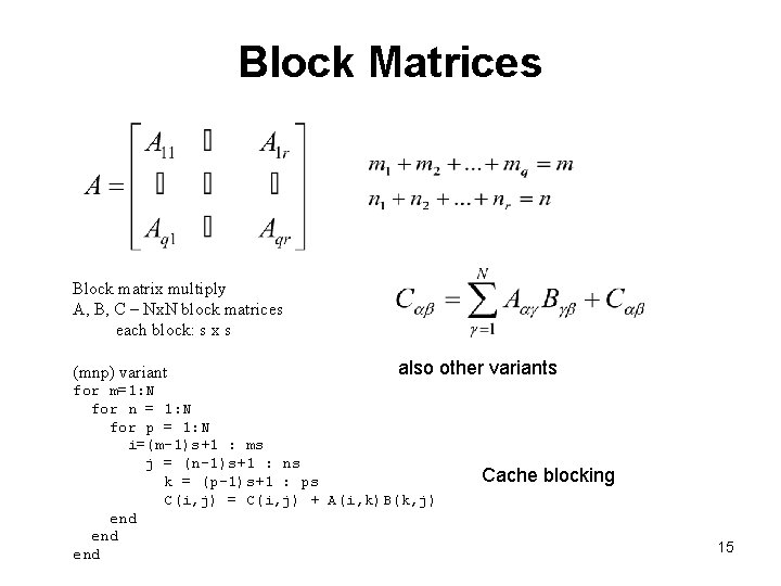
Block Matrices Block matrix multiply A, B, C – Nx. N block matrices each block: s x s (mnp) variant also other variants for m=1: N for n = 1: N for p = 1: N i=(m-1)s+1 : ms j = (n-1)s+1 : ns k = (p-1)s+1 : ps C(i, j) = C(i, j) + A(i, k)B(k, j) end end Cache blocking 15

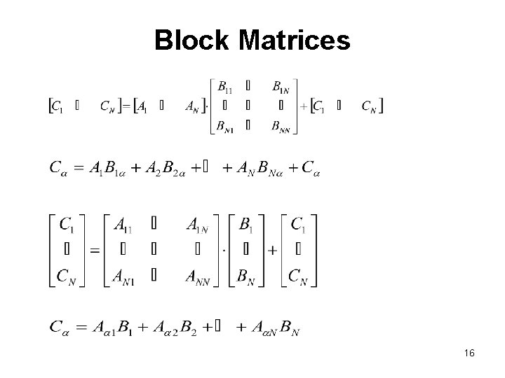
Block Matrices 16

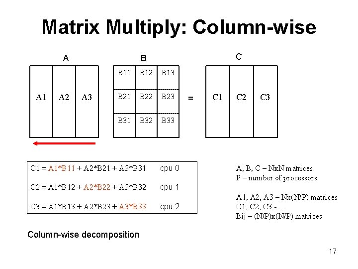
Matrix Multiply: Column-wise A A 1 A 2 C B A 3 B 11 B 12 B 13 B 21 B 22 B 23 B 31 B 32 B 33 C 1 = A 1*B 11 + A 2*B 21 + A 3*B 31 cpu 0 C 2 = A 1*B 12 + A 2*B 22 + A 3*B 32 cpu 1 C 3 = A 1*B 13 + A 2*B 23 + A 3*B 33 cpu 2 = C 1 C 2 C 3 A, B, C – Nx. N matrices P – number of processors A 1, A 2, A 3 – Nx(N/P) matrices C 1, C 2, C 3 - … Bij – (N/P)x(N/P) matrices Column-wise decomposition 17

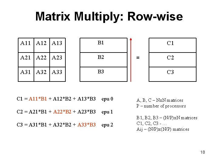
Matrix Multiply: Row-wise A 11 A 12 A 13 B 1 A 22 A 23 B 2 A 31 A 32 A 33 B 3 C 1 = A 11*B 1 + A 12*B 2 + A 13*B 3 cpu 0 C 2 = A 21*B 1 + A 22*B 2 + A 23*B 3 cpu 1 C 3 = A 31*B 1 + A 32*B 2 + A 33*B 3 cpu 2 C 1 = C 2 C 3 A, B, C – Nx. N matrices P – number of processors B 1, B 2, B 3 – (N/P)x. N matrices C 1, C 2, C 3 - … Aij – (N/P)x(N/P) matrices 18

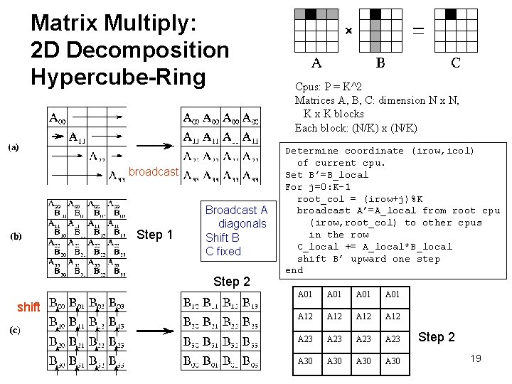
Matrix Multiply: 2 D Decomposition Hypercube-Ring broadcast Step 1 Broadcast A diagonals Shift B C fixed Step 2 shift Cpus: P = K^2 Matrices A, B, C: dimension N x N, K x K blocks Each block: (N/K) x (N/K) Determine coordinate (irow, icol) of current cpu. Set B’=B_local For j=0: K-1 root_col = (irow+j)%K broadcast A’=A_local from root cpu (irow, root_col) to other cpus in the row C_local += A_local*B_local shift B’ upward one step end A 01 A 12 A 23 A 30 Step 2 19

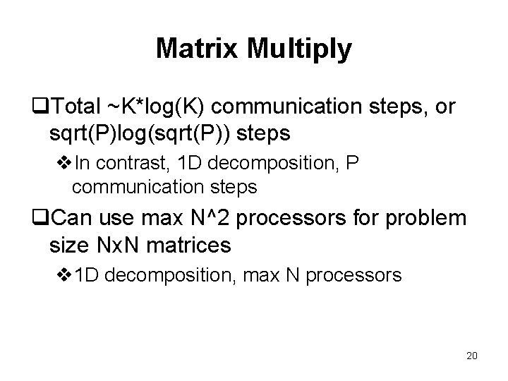
Matrix Multiply q. Total ~K*log(K) communication steps, or sqrt(P)log(sqrt(P)) steps v. In contrast, 1 D decomposition, P communication steps q. Can use max N^2 processors for problem size Nx. N matrices v 1 D decomposition, max N processors 20

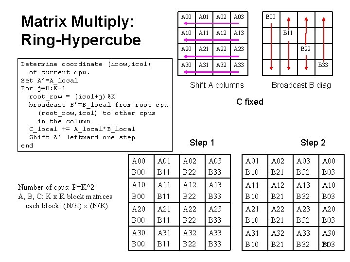
Matrix Multiply: Ring-Hypercube A 00 A 01 A 02 A 03 A 10 A 11 A 12 A 13 A 20 A 21 A 22 A 23 Determine coordinate (irow, icol) of current cpu. Set A’=A_local For j=0: K-1 root_row = (icol+j)%K broadcast B’=B_local from root cpu (root_row, icol) to other cpus in the column C_local += A_local*B_local Shift A’ leftward one step end A 30 A 31 A 32 A 33 Number of cpus: P=K^2 A, B, C: K x K block matrices each block: (N/K) x (N/K) B 00 B 11 B 22 B 33 Shift A columns Broadcast B diag C fixed Step 1 Step 2 A 00 B 00 A 01 B 11 A 02 B 22 A 03 B 33 A 01 B 10 A 02 B 21 A 03 B 32 A 00 B 03 A 10 B 00 A 11 B 11 A 12 B 22 A 13 B 33 A 11 B 10 A 12 B 21 A 13 B 32 A 10 B 03 A 20 B 00 A 21 B 11 A 22 B 22 A 23 B 33 A 21 B 10 A 22 B 21 A 23 B 32 A 20 B 03 A 30 B 00 A 31 B 11 A 32 B 22 A 33 B 33 A 31 B 10 A 32 B 21 A 33 B 32 A 30 B 03 21

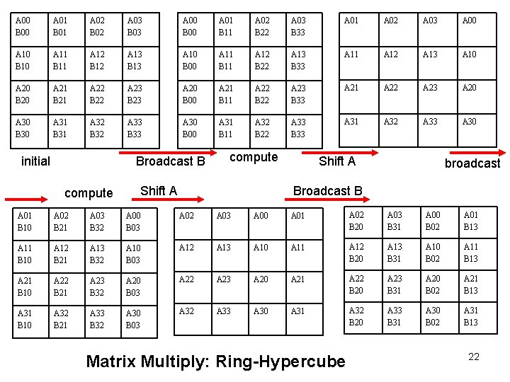
A 00 B 00 A 01 B 01 A 02 B 02 A 03 B 03 A 00 B 00 A 01 B 11 A 02 B 22 A 03 B 33 A 01 A 02 A 03 A 00 A 10 B 10 A 11 B 11 A 12 B 12 A 13 B 13 A 10 B 00 A 11 B 11 A 12 B 22 A 13 B 33 A 11 A 12 A 13 A 10 A 20 B 20 A 21 B 21 A 22 B 22 A 23 B 23 A 20 B 00 A 21 B 11 A 22 B 22 A 23 B 33 A 21 A 22 A 23 A 20 A 30 B 30 A 31 B 31 A 32 B 32 A 33 B 33 A 30 B 00 A 31 B 11 A 32 B 22 A 33 B 33 A 31 A 32 A 33 A 30 initial Broadcast B compute Shift A broadcast B A 01 B 10 A 02 B 21 A 03 B 32 A 00 B 03 A 02 A 03 A 00 A 01 A 02 B 20 A 03 B 31 A 00 B 02 A 01 B 13 A 11 B 10 A 12 B 21 A 13 B 32 A 10 B 03 A 12 A 13 A 10 A 11 A 12 B 20 A 13 B 31 A 10 B 02 A 11 B 13 A 21 B 10 A 22 B 21 A 23 B 32 A 20 B 03 A 22 A 23 A 20 A 21 A 22 B 20 A 23 B 31 A 20 B 02 A 21 B 13 A 31 B 10 A 32 B 21 A 33 B 32 A 30 B 03 A 32 A 33 A 30 A 31 A 32 B 20 A 33 B 31 A 30 B 02 A 31 B 13 Matrix Multiply: Ring-Hypercube 22

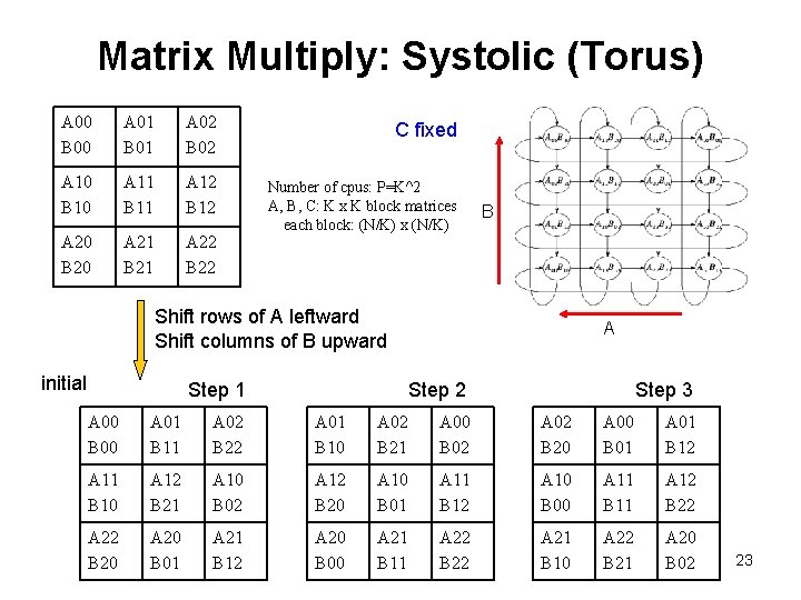
Matrix Multiply: Systolic (Torus) A 00 B 00 A 01 B 01 A 02 B 02 C fixed A 10 B 10 A 11 B 11 A 12 B 12 A 20 B 20 A 21 B 21 A 22 B 22 Number of cpus: P=K^2 A, B, C: K x K block matrices each block: (N/K) x (N/K) B Shift rows of A leftward Shift columns of B upward initial Step 1 A Step 2 Step 3 A 00 B 00 A 01 B 11 A 02 B 22 A 01 B 10 A 02 B 21 A 00 B 02 A 02 B 20 A 00 B 01 A 01 B 12 A 11 B 10 A 12 B 21 A 10 B 02 A 12 B 20 A 10 B 01 A 11 B 12 A 10 B 00 A 11 B 11 A 12 B 22 A 22 B 20 A 20 B 01 A 21 B 12 A 20 B 00 A 21 B 11 A 22 B 22 A 21 B 10 A 22 B 21 A 20 B 02 23

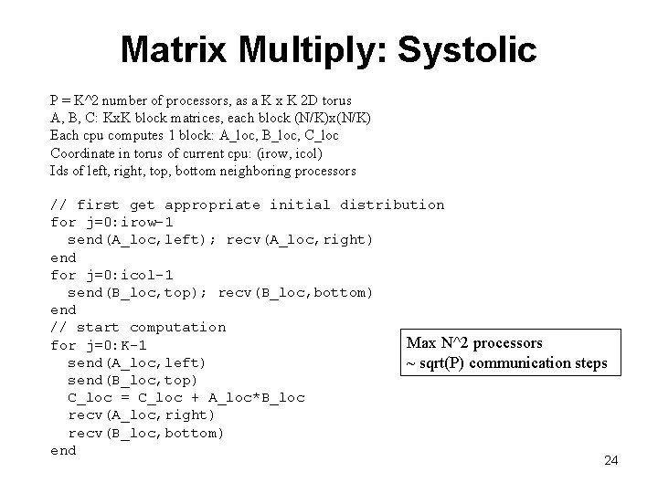
Matrix Multiply: Systolic P = K^2 number of processors, as a K x K 2 D torus A, B, C: Kx. K block matrices, each block (N/K)x(N/K) Each cpu computes 1 block: A_loc, B_loc, C_loc Coordinate in torus of current cpu: (irow, icol) Ids of left, right, top, bottom neighboring processors // first get appropriate initial distribution for j=0: irow-1 send(A_loc, left); recv(A_loc, right) end for j=0: icol-1 send(B_loc, top); recv(B_loc, bottom) end // start computation Max N^2 processors for j=0: K-1 send(A_loc, left) ~ sqrt(P) communication steps send(B_loc, top) C_loc = C_loc + A_loc*B_loc recv(A_loc, right) recv(B_loc, bottom) end 24

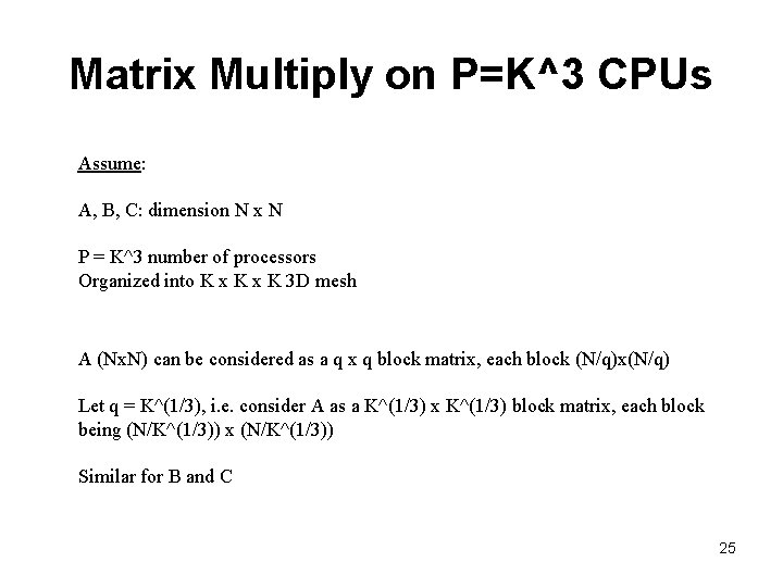
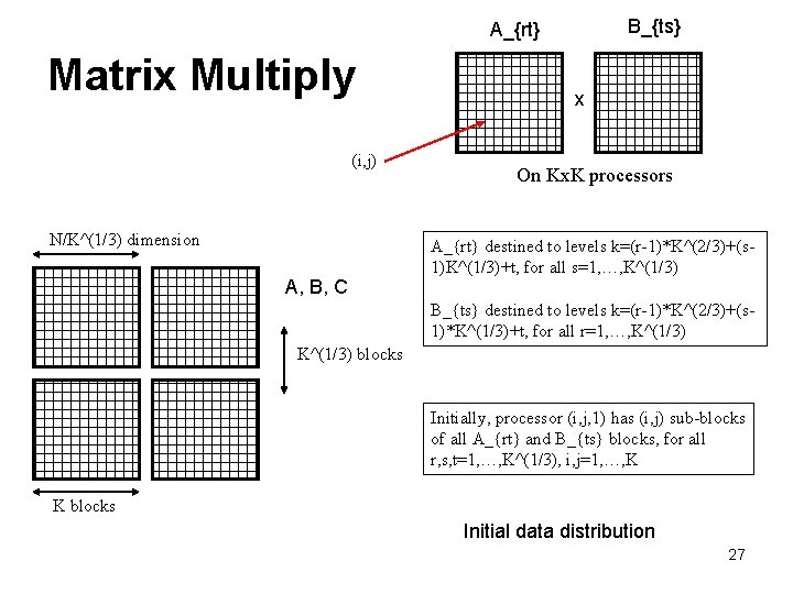
Matrix Multiply on P=K^3 CPUs Assume: A, B, C: dimension N x N P = K^3 number of processors Organized into K x K 3 D mesh A (Nx. N) can be considered as a q x q block matrix, each block (N/q)x(N/q) Let q = K^(1/3), i. e. consider A as a K^(1/3) x K^(1/3) block matrix, each block being (N/K^(1/3)) x (N/K^(1/3)) Similar for B and C 25

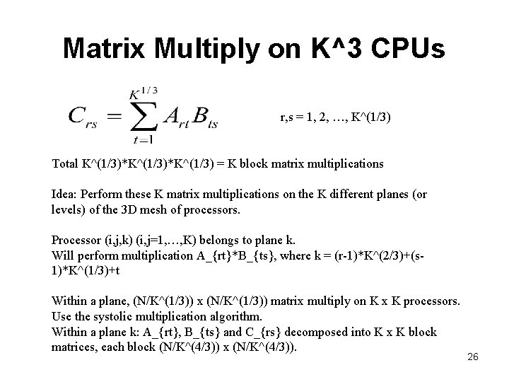
Matrix Multiply on K^3 CPUs r, s = 1, 2, …, K^(1/3) Total K^(1/3)*K^(1/3) = K block matrix multiplications Idea: Perform these K matrix multiplications on the K different planes (or levels) of the 3 D mesh of processors. Processor (i, j, k) (i, j=1, …, K) belongs to plane k. Will perform multiplication A_{rt}*B_{ts}, where k = (r-1)*K^(2/3)+(s 1)*K^(1/3)+t Within a plane, (N/K^(1/3)) x (N/K^(1/3)) matrix multiply on K x K processors. Use the systolic multiplication algorithm. Within a plane k: A_{rt}, B_{ts} and C_{rs} decomposed into K x K block matrices, each block (N/K^(4/3)) x (N/K^(4/3)). 26

B_{ts} A_{rt} Matrix Multiply (i, j) N/K^(1/3) dimension A, B, C x On Kx. K processors A_{rt} destined to levels k=(r-1)*K^(2/3)+(s 1)K^(1/3)+t, for all s=1, …, K^(1/3) B_{ts} destined to levels k=(r-1)*K^(2/3)+(s 1)*K^(1/3)+t, for all r=1, …, K^(1/3) blocks Initially, processor (i, j, 1) has (i, j) sub-blocks of all A_{rt} and B_{ts} blocks, for all r, s, t=1, …, K^(1/3), i, j=1, …, K K blocks Initial data distribution 27

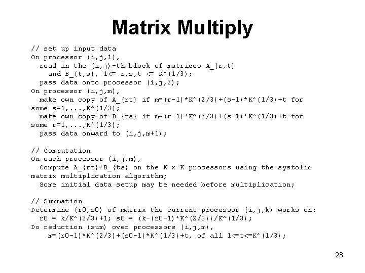
Matrix Multiply // set up input data On processor (i, j, 1), read in the (i, j)-th block of matrices A_{r, t} and B_{t, s}, 1<= r, s, t <= K^(1/3); pass data onto processor (i, j, 2); On processor (i, j, m), make own copy of A_{rt} if m=(r-1)*K^(2/3)+(s-1)*K^(1/3)+t for some s=1, . . . , K^(1/3); make own copy of B_{ts} if m=(r-1)*K^(2/3)+(s-1)*K^(1/3)+t for some r=1, . . . , K^(1/3); pass data onward to (i, j, m+1); // Computation On each processor (i, j, m), Compute A_{rt}*B_{ts} on the K x K processors using the systolic matrix multiplication algorithm; Some initial data setup may be needed before multiplication; // Summation Determine (r 0, s 0) of matrix the current processor (i, j, k) works on: r 0 = k/K^(2/3)+1; s 0 = (k-(r 0 -1)*K^(2/3))/K^(1/3); Do reduction (sum) over processors (i, j, m), m=(r 0 -1)*K^(2/3)+(s 0 -1)*K^(1/3)+t, of all 1<=t<=K^(1/3); 28

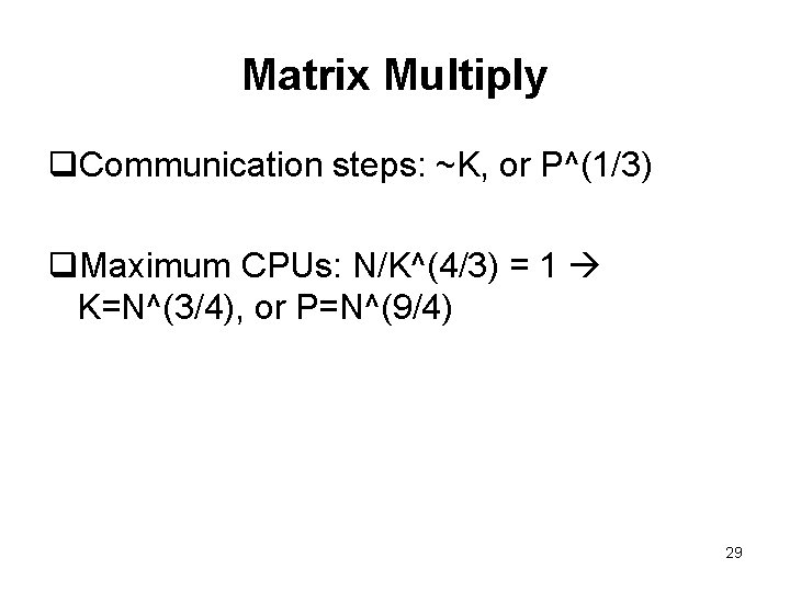
Matrix Multiply q. Communication steps: ~K, or P^(1/3) q. Maximum CPUs: N/K^(4/3) = 1 K=N^(3/4), or P=N^(9/4) 29

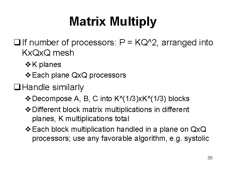
Matrix Multiply q If number of processors: P = KQ^2, arranged into Kx. Q mesh v. K planes v. Each plane Qx. Q processors q Handle similarly v. Decompose A, B, C into K^(1/3)x. K^(1/3) blocks v. Different block matrix multiplications in different planes, K multiplications total v. Each block multiplication handled in a plane on Qx. Q processors; use any favorable algorithm, e. g. systolic 30

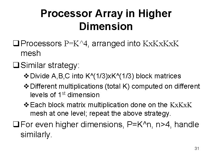
Processor Array in Higher Dimension q Processors P=K^4, arranged into Kx. Kx. K mesh q Similar strategy: v. Divide A, B, C into K^(1/3)x. K^(1/3) block matrices v. Different multiplications (total K) computed on different levels of 1 st dimension v. Each block matrix multiplication done on the Kx. K mesh at one level; repeat the above strategy. q For even higher dimensions, P=K^n, n>4, handle similarly. 31

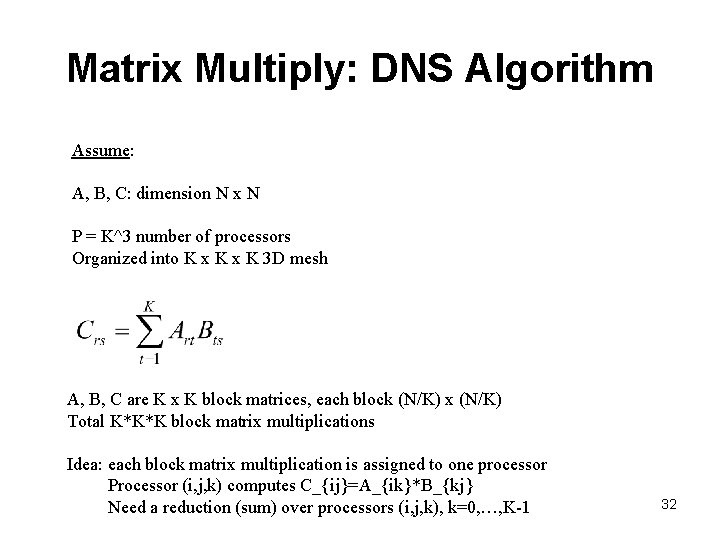
Matrix Multiply: DNS Algorithm Assume: A, B, C: dimension N x N P = K^3 number of processors Organized into K x K 3 D mesh A, B, C are K x K block matrices, each block (N/K) x (N/K) Total K*K*K block matrix multiplications Idea: each block matrix multiplication is assigned to one processor Processor (i, j, k) computes C_{ij}=A_{ik}*B_{kj} Need a reduction (sum) over processors (i, j, k), k=0, …, K-1 32

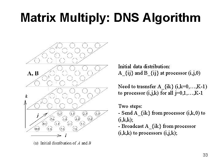
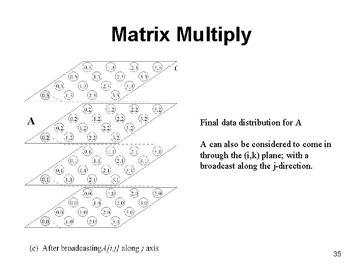
Matrix Multiply: DNS Algorithm Initial data distribution: A_{ij} and B_{ij} at processor (i, j, 0) Need to trasnsfer A_{ik} (i, k=0, …, K-1) to processor (i, j, k) for all j=0, 1, …, K-1 Two steps: - Send A_{ik} from processor (i, k, 0) to (i, k, k); - Broadcast A_{ik} from processor (i, k, k) to processors (i, j, k); 33

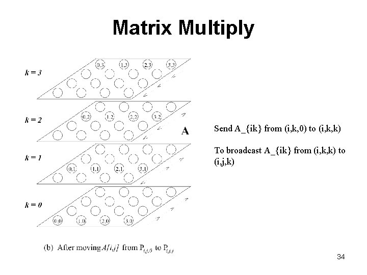
Matrix Multiply Send A_{ik} from (i, k, 0) to (i, k, k) To broadcast A_{ik} from (i, k, k) to (i, j, k) 34

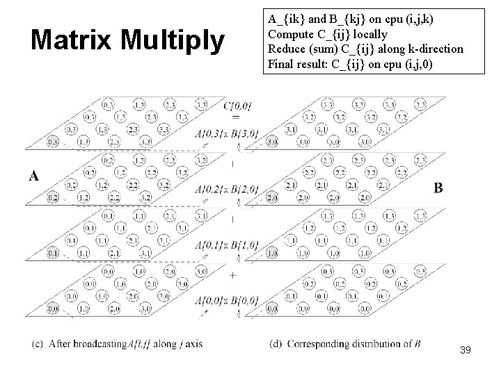
Matrix Multiply Final data distribution for A A can also be considered to come in through the (i, k) plane; with a broadcast along the j-direction. 35

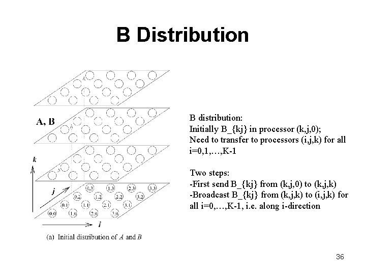
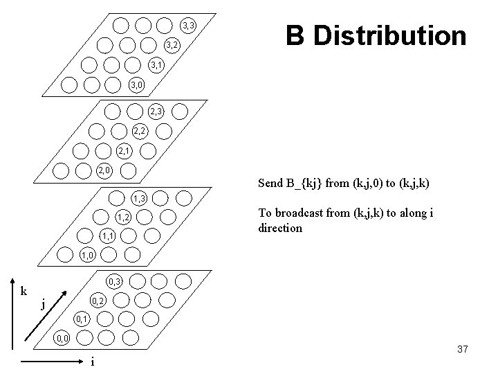
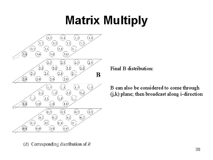
B Distribution B distribution: Initially B_{kj} in processor (k, j, 0); Need to transfer to processors (i, j, k) for all i=0, 1, …, K-1 Two steps: -First send B_{kj} from (k, j, 0) to (k, j, k) -Broadcast B_{kj} from (k, j, k) to (i, j, k) for all i=0, …, K-1, i. e. along i-direction 36

3, 3 3, 2 B Distribution 3, 1 3, 0 2, 3 2, 2 2, 1 2, 0 Send B_{kj} from (k, j, 0) to (k, j, k) 1, 3 1, 2 1, 1 To broadcast from (k, j, k) to along i direction 1, 0 k 0, 3 j 0, 2 0, 1 0, 0 37 i

Matrix Multiply Final B distribution: B can also be considered to come through (j, k) plane; then broadcast along i-direction 38

Matrix Multiply A_{ik} and B_{kj} on cpu (i, j, k) Compute C_{ij} locally Reduce (sum) C_{ij} along k-direction Final result: C_{ij} on cpu (i, j, 0) 39

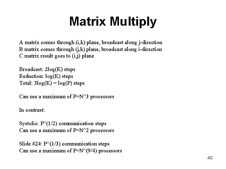
Matrix Multiply A matrix comes through (i, k) plane, broadcast along j-direction B matrix comes through (j, k) plane, broadcast along i-direction C matrix result goes to (i, j) plane Broadcast: 2 log(K) steps Reduction: log(K) steps Total: 3 log(K) = log(P) steps Can use a maximum of P=N^3 processors In contrast: Systolic: P^(1/2) communication steps Can use a maximum of P=N^2 processors Slide #24: P^(1/3) communication steps Can use a maximum of P=N^(9/4) processors 40