Un universo tridimensional con Gaia Francesca Figueras On

Un universo tridimensional con Gaia Francesca Figueras On behalf of the UB- Gaia team Universidad de Barcelona (Spain)

Index • • Basic principles and data reduction strategy What Gaia will observe: the Gaia Simulator (GUMS and GOG) Scientific challenges: some examples On ground spectroscopic surveys complementary to Gaia

Gaia astrometric accuracy

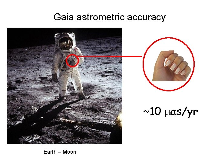
Gaia astrometric accuracy ~10 as/yr Earth – Moon

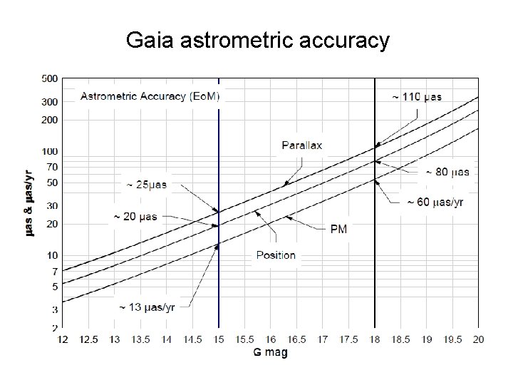
Gaia astrometric accuracy

Basic Principles

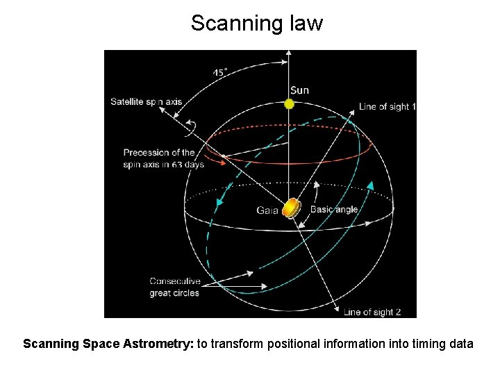
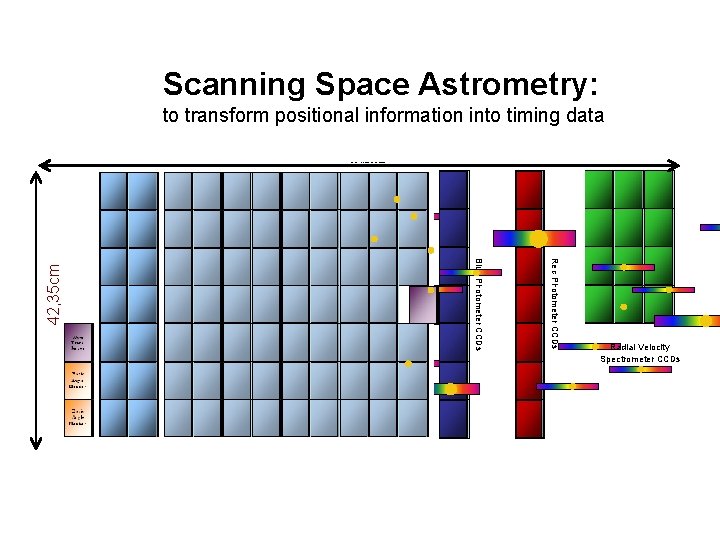
Scanning law Scanning Space Astrometry: to transform positional information into timing data

Scanning Space Astrometry: Red Photometer CCDs Blue Photometer CCDs 42, 35 cm to transform positional information into timing data Radial Velocity Spectrometer CCDs

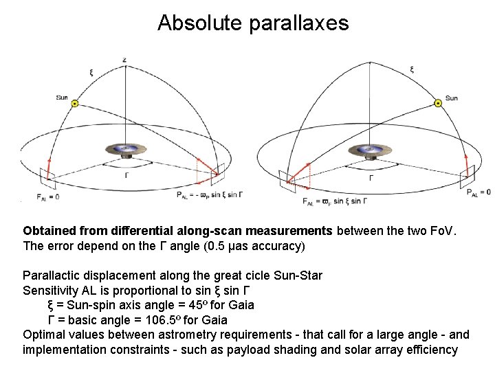
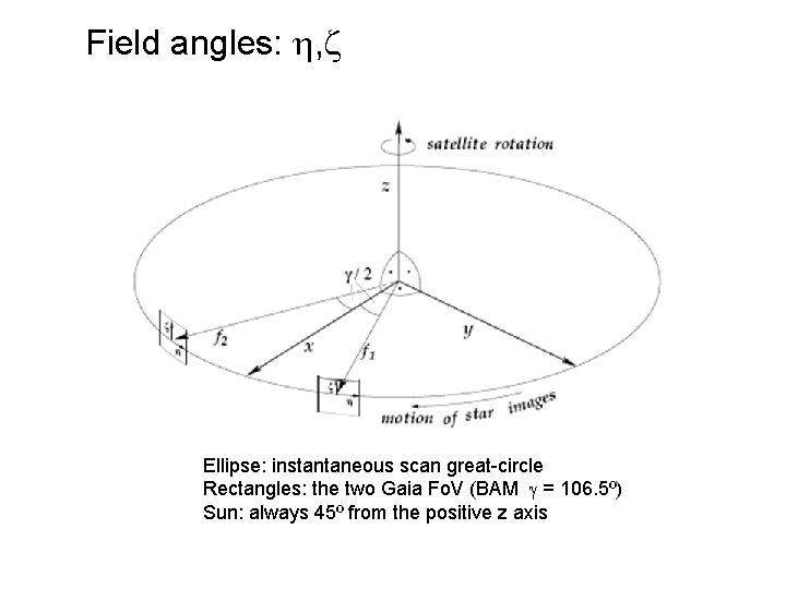
Absolute parallaxes Obtained from differential along-scan measurements between the two Fo. V. The error depend on the Γ angle (0. 5 μas accuracy) Parallactic displacement along the great cicle Sun-Star Sensitivity AL is proportional to sin ξ sin Γ ξ = Sun-spin axis angle = 45º for Gaia Γ = basic angle = 106. 5º for Gaia Optimal values between astrometry requirements - that call for a large angle - and implementation constraints - such as payload shading and solar array efficiency

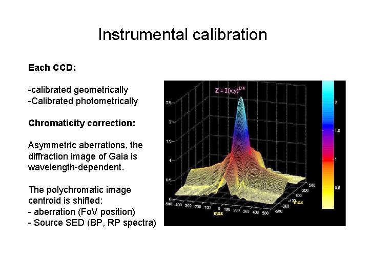
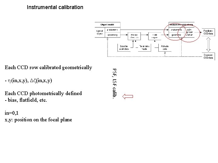
Instrumental calibration Each CCD: -calibrated geometrically -Calibrated photometrically Chromaticity correction: Asymmetric aberrations, the diffraction image of Gaia is wavelength-dependent. The polychromatic image centroid is shifted: - aberration (Fo. V position) - Source SED (BP, RP spectra)

Reduction Strategy

AGIS Core Processing 100 million “well-behaved” stars

Intermediate Data Update

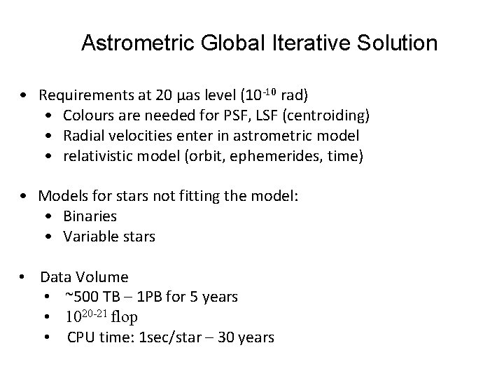
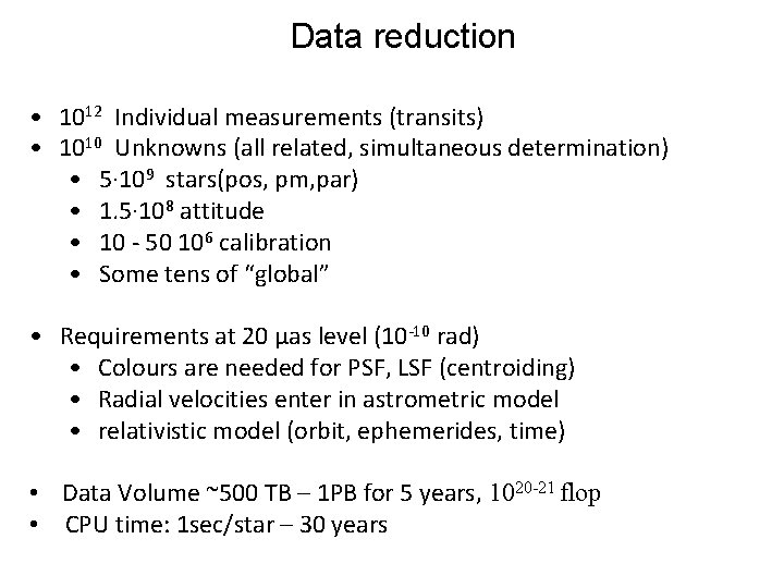
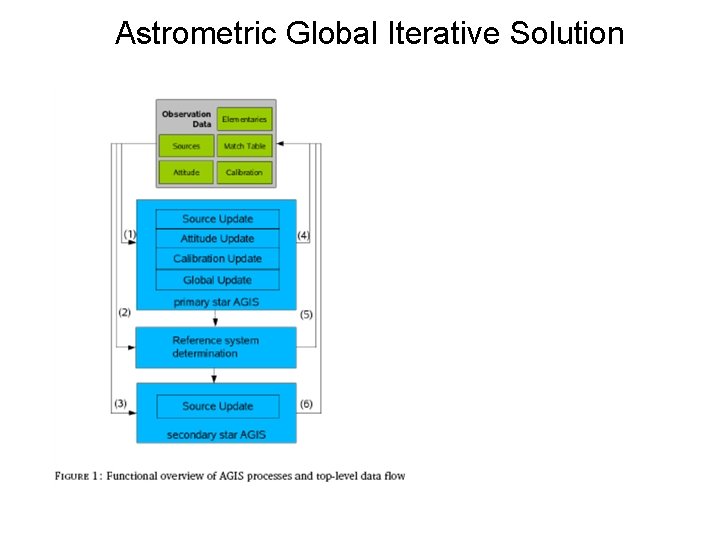
Astrometric Global Iterative Solution • Requirements at 20 μas level (10 -10 rad) • Colours are needed for PSF, LSF (centroiding) • Radial velocities enter in astrometric model • relativistic model (orbit, ephemerides, time) • Models for stars not fitting the model: • Binaries • Variable stars • Data Volume • ~500 TB – 1 PB for 5 years • 1020 -21 flop • CPU time: 1 sec/star – 30 years

What Gaia will observe? the Gaia Simulator: GUMS and GOG

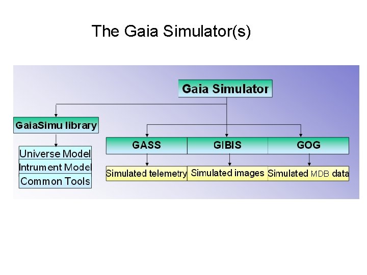
The Gaia Simulator(s)

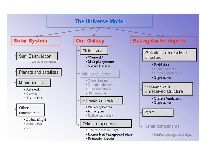
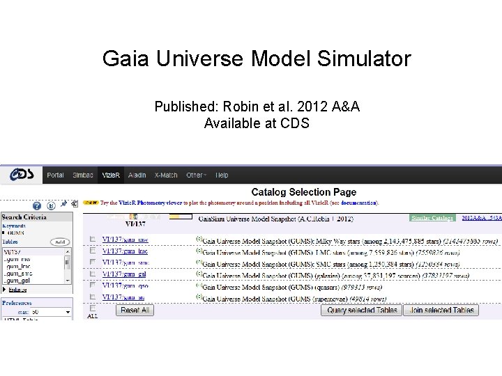
Gaia Universe Model Simulator Published: Robin et al. 2012 A&A Available at CDS

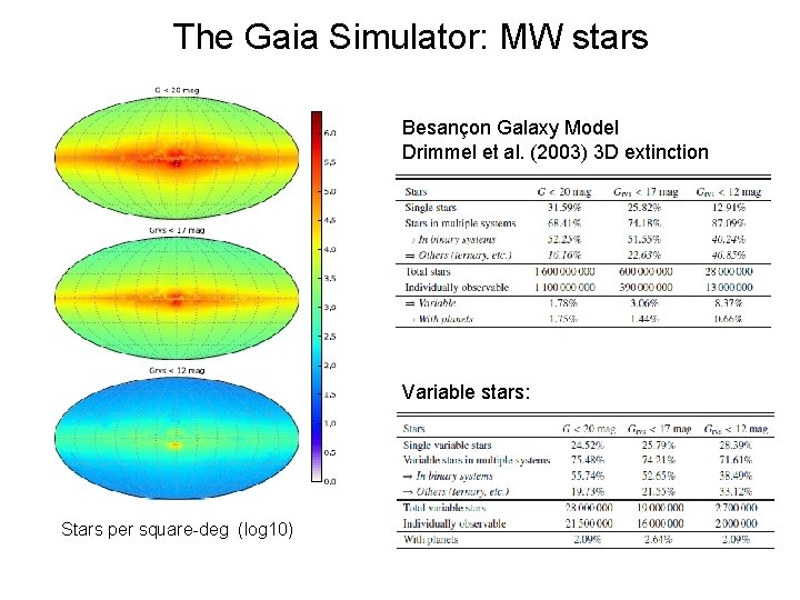
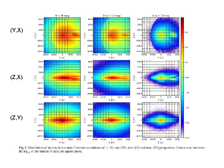
The Gaia Simulator: MW stars Besançon Galaxy Model Drimmel et al. (2003) 3 D extinction Variable stars: Stars per square-deg (log 10)

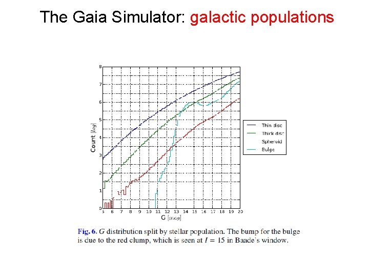
The Gaia Simulator: galactic populations

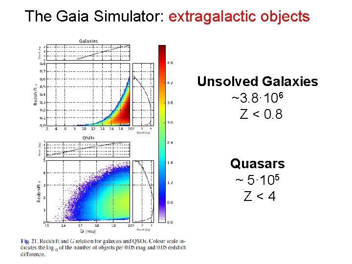
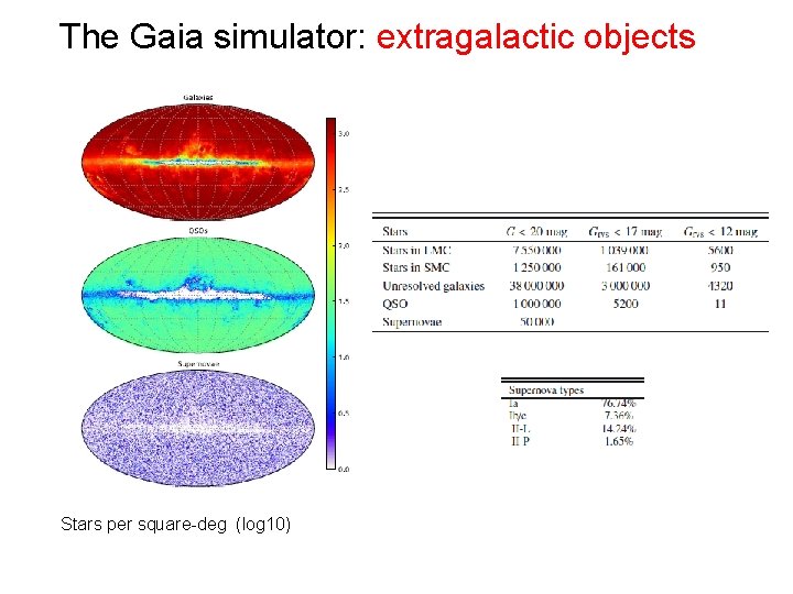
The Gaia Simulator: extragalactic objects Unsolved Galaxies ~3. 8· 106 Z < 0. 8 Quasars ~ 5· 105 Z<4

GOG: Gaia Object Generator An attempt to simulate Gaia products GUMS + a model for Gaia errors Goals: To fill the Gaia Archive For Science Exploitation

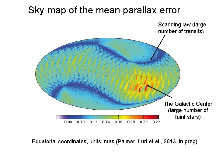
Sky map of the mean parallax error Scanning law (large number of transits) The Galactic Center (large number of faint stars) Equatorial coordinates, units: mas (Palmer, Luri et al. , 2013, in prep)

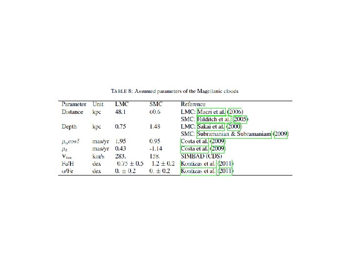
Gaia and the Magellanic Clouds

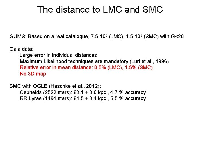
The distance to LMC and SMC GUMS: Based on a real catalogue, 7. 5· 106 (LMC), 1. 5 106 (SMC) with G<20 Gaia data: Large error in individual distances Maximum Likelihood techniques are mandatory (Luri et al. , 1996) Relative error in mean distance: 0. 5% (LMC), 1. 5% (SMC) No 3 D map SMC with OGLE (Haschke et al. , 2012): Cepheids (2522 stars): 63. 1 3. 0 kpc , 4. 7 % accuracy RR Lyrae (1494 stars): 61. 5 3. 4 kpc , 5. 5 % accuracy

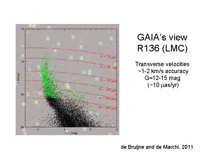
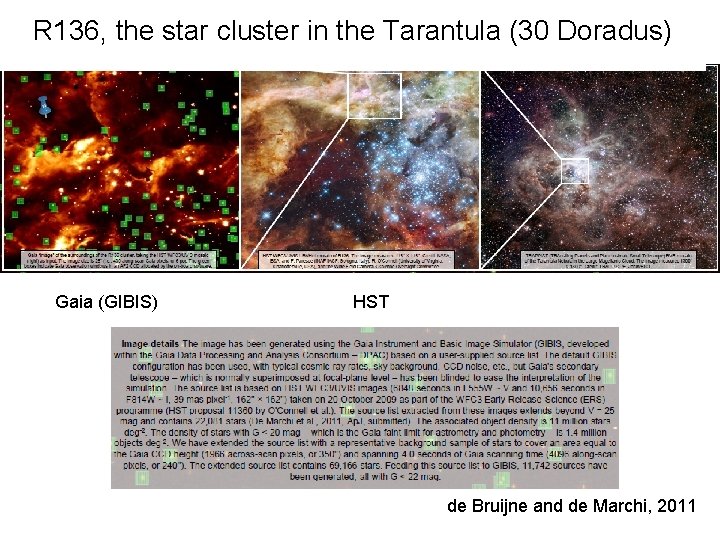
GAIA’s view R 136 (LMC) Transverse velocities ~1 -2 km/s accuracy G=12 -15 mag (~10 as/yr) de Bruijne and de Marchi, 2011

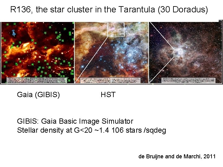
R 136, the star cluster in the Tarantula (30 Doradus) Gaia (GIBIS) HST GIBIS: Gaia Basic Image Simulator Stellar density at G<20 ~1. 4 106 stars /sqdeg de Bruijne and de Marchi, 2011

Gaia and the distance scale

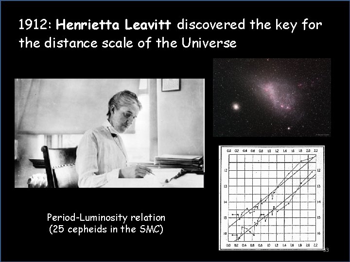
1912: Henrietta Leavitt discovered the key for the distance scale of the Universe Period-Luminosity relation (25 cepheids in the SMC) 33

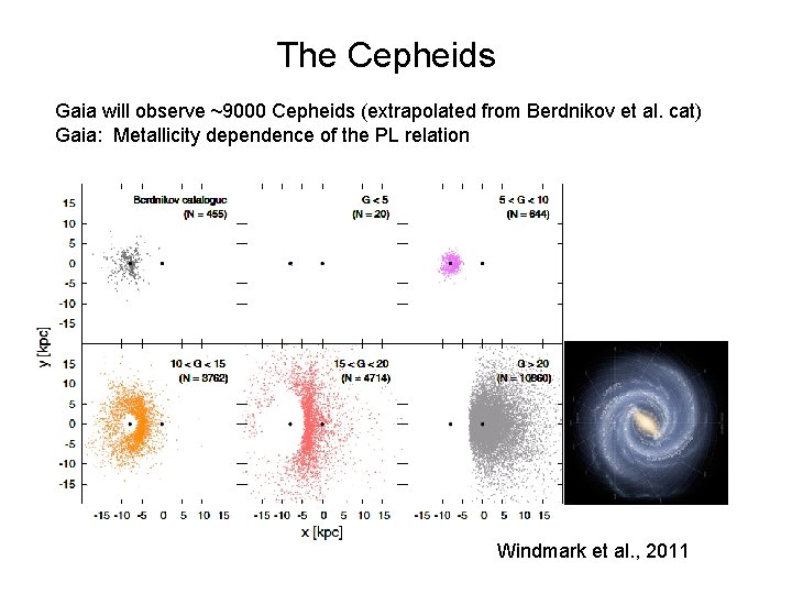
The Cepheids Gaia will observe ~9000 Cepheids (extrapolated from Berdnikov et al. cat) Gaia: Metallicity dependence of the PL relation Windmark et al. , 2011

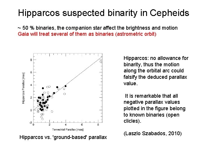
Hipparcos suspected binarity in Cepheids ~ 50 % binaries, the companion star affect the brightness and motion Gaia will treat several of them as binaries (astrometric orbit) Hipparcos: no allowance for binarity, thus the motion along the orbital arc could falsify the deduced parallax value. It is remarkable that all negative parallax values plotted in the figure belong to known binaries (open clicles). Hipparcos vs. 'ground-based' parallax (Laszlo Szabados, 2010)

~500 000 Quasars - The Reference Frame - How to detect them? - Lensed QSO in Gaia survey? - Astrometry for astrophysics -…

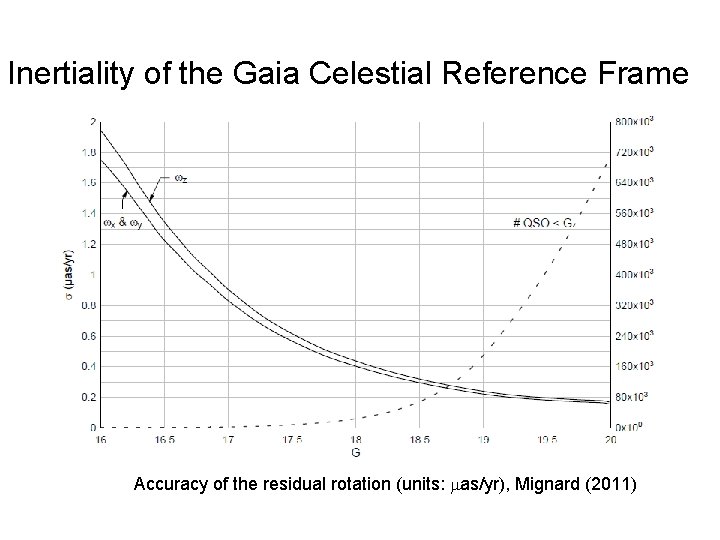
Inertiality of the Gaia Celestial Reference Frame Accuracy of the residual rotation (units: as/yr), Mignard (2011)

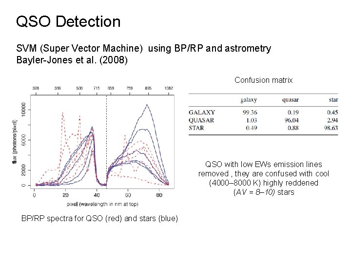
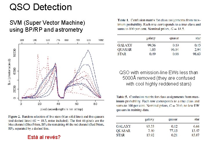
QSO Detection SVM (Super Vector Machine) using BP/RP and astrometry Bayler-Jones et al. (2008) Confusion matrix QSO with low EWs emission lines removed , they are confused with cool (4000– 8000 K) highly reddened (AV = 8– 10) stars BP/RP spectra for QSO (red) and stars (blue)

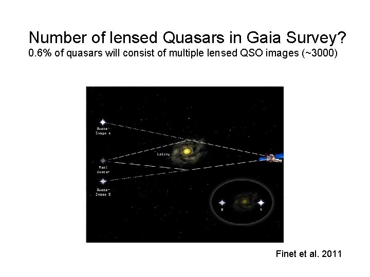
Number of lensed Quasars in Gaia Survey? 0. 6% of quasars will consist of multiple lensed QSO images (~3000) Finet et al. 2011

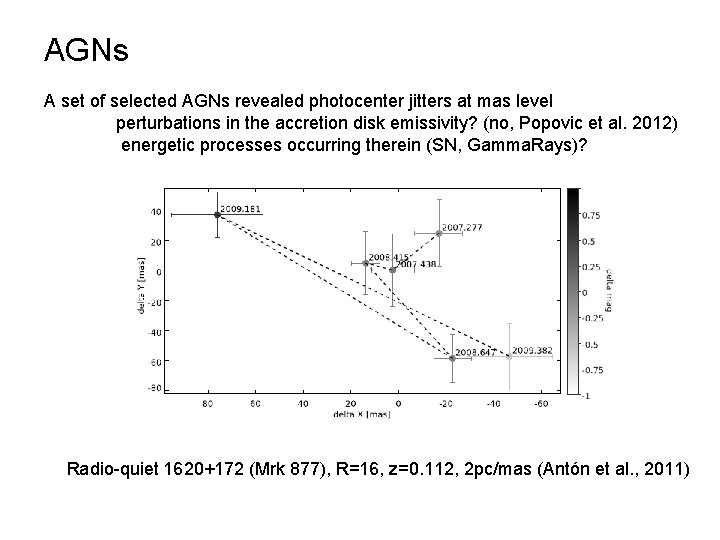
AGNs A set of selected AGNs revealed photocenter jitters at mas level perturbations in the accretion disk emissivity? (no, Popovic et al. 2012) energetic processes occurring therein (SN, Gamma. Rays)? Radio-quiet 1620+172 (Mrk 877), R=16, z=0. 112, 2 pc/mas (Antón et al. , 2011)

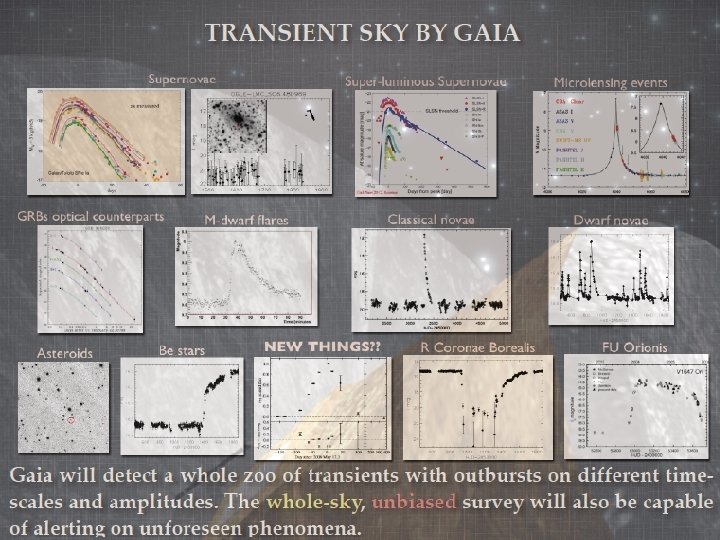
The transient sky by Gaia Ground contact: 8 h /day Analysis and anomaly detection at Cambridge Alerts issued in 24 -48 hours after observations See: Wyrzykowski et al. 2013, IAU 298

The Red Clump Stars The Galactic Bar (s) and the Spirals

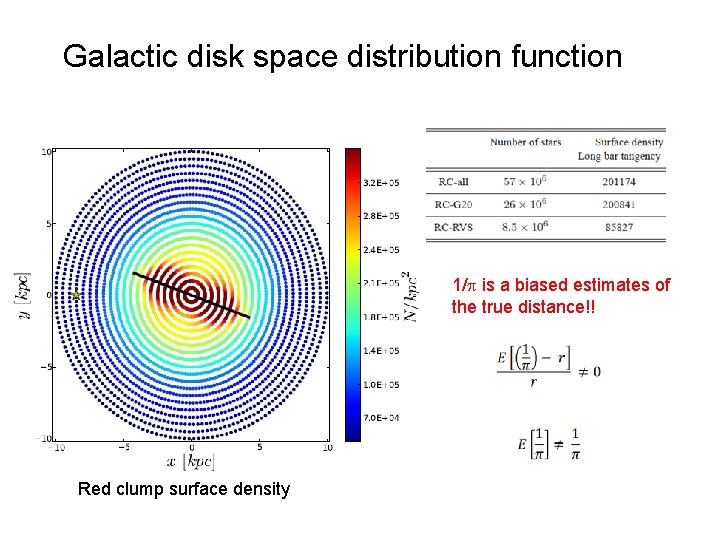
Galactic disk space distribution function 1/ is a biased estimates of the true distance!! Red clump surface density

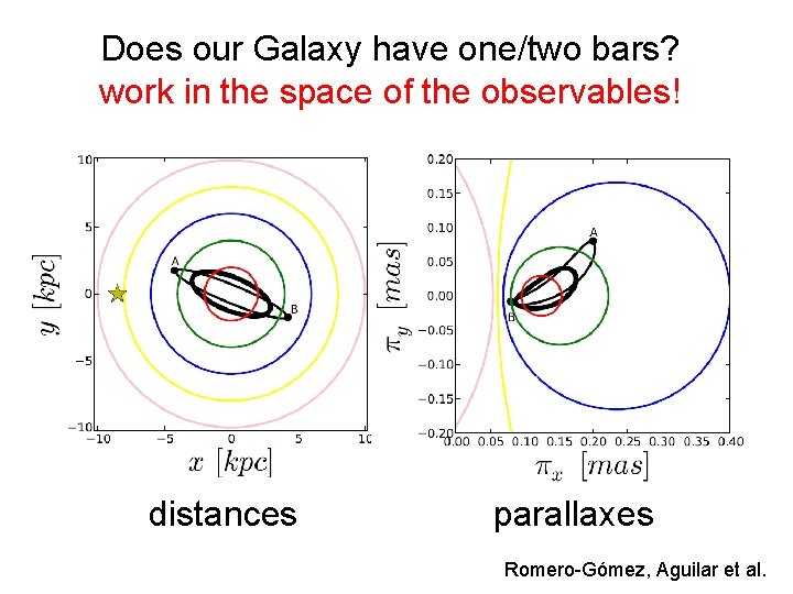
Does our Galaxy have one/two bars? work in the space of the observables! distances parallaxes Romero-Gómez, Aguilar et al.

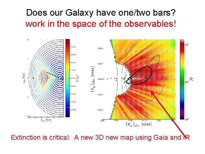
Does our Galaxy have one/two bars? work in the space of the observables! Extinction is critical: A new 3 D new map using Gaia and IR

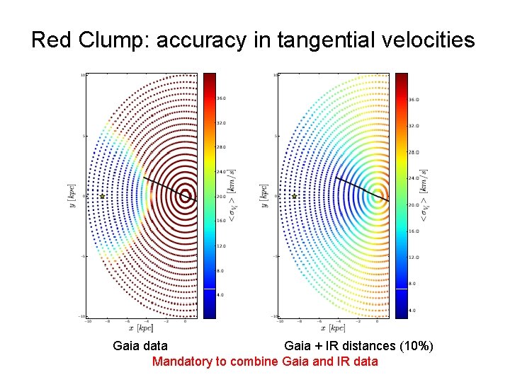
Red Clump: accuracy in tangential velocities Gaia data Gaia + IR distances (10%) Mandatory to combine Gaia and IR data

Hyper-Runaway Stars

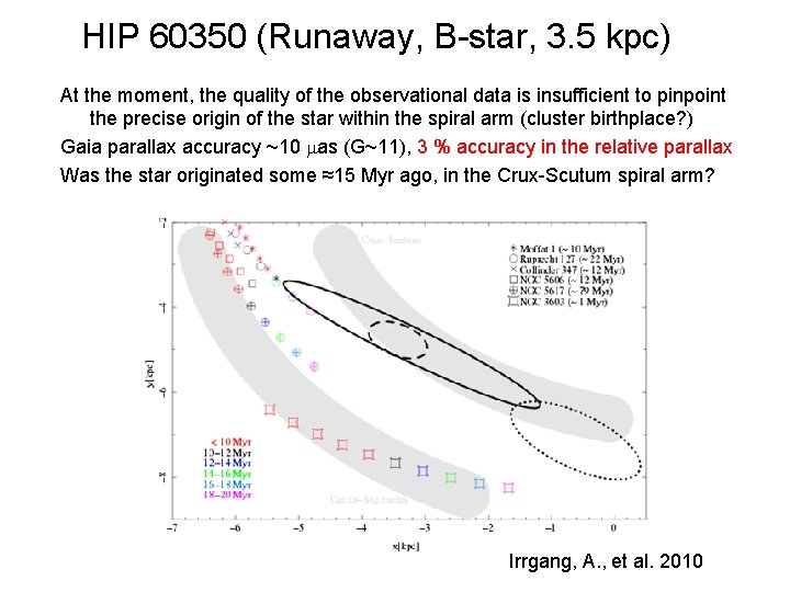
HIP 60350 (Runaway, B-star, 3. 5 kpc) At the moment, the quality of the observational data is insufficient to pinpoint the precise origin of the star within the spiral arm (cluster birthplace? ) Gaia parallax accuracy ~10 as (G~11), 3 % accuracy in the relative parallax Was the star originated some ≈15 Myr ago, in the Crux-Scutum spiral arm? Irrgang, A. , et al. 2010

Solar System minor bodies ~100 TNO: orbit, binarity detection, … ~2· 105 asteroids: orbit, rotation, shape, … Can Gaia discover new Earth Trojans?

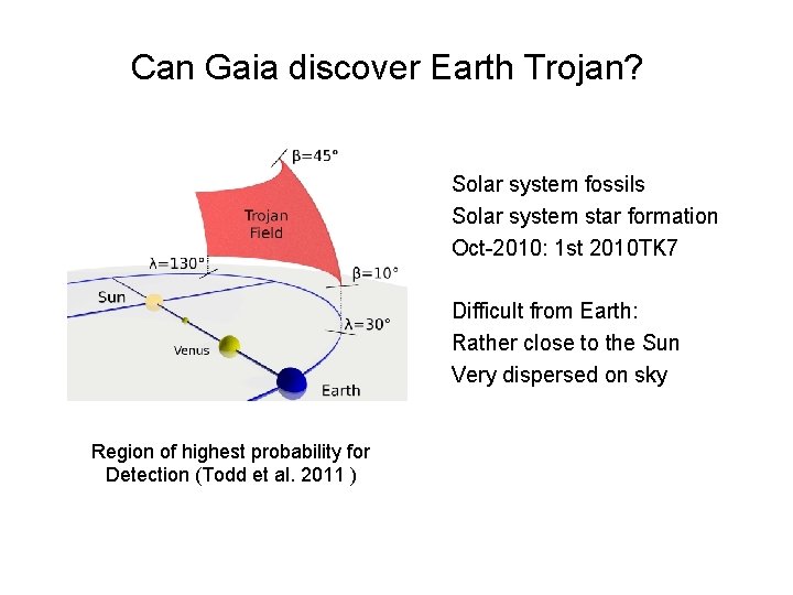
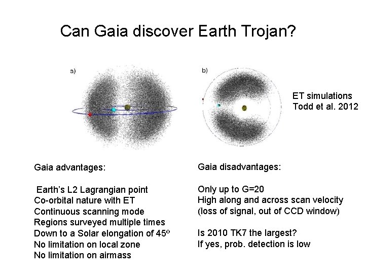
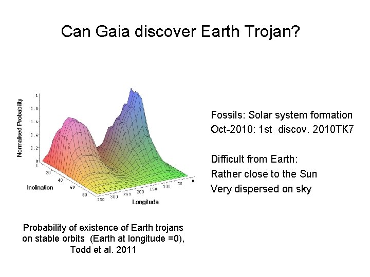
Can Gaia discover Earth Trojan? Solar system fossils Solar system star formation Oct-2010: 1 st 2010 TK 7 Difficult from Earth: Rather close to the Sun Very dispersed on sky Region of highest probability for Detection (Todd et al. 2011 )

Can Gaia discover Earth Trojan? ET simulations Todd et al. 2012 Gaia advantages: Gaia disadvantages: Earth’s L 2 Lagrangian point Co-orbital nature with ET Continuous scanning mode Regions surveyed multiple times Down to a Solar elongation of 45º No limitation on local zone No limitation on airmass Only up to G=20 High along and across scan velocity (loss of signal, out of CCD window) Is 2010 TK 7 the largest? If yes, prob. detection is low

On-ground Spectroscopic Surveys complementary to Gaia

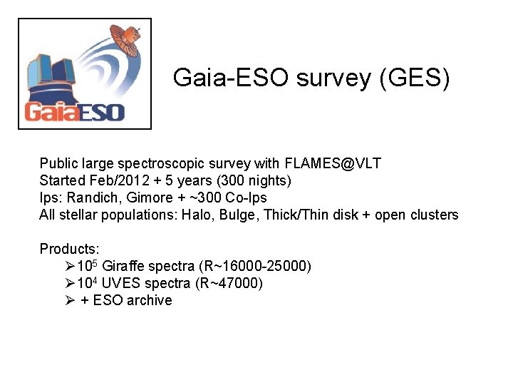
Gaia-ESO survey (GES) Public large spectroscopic survey with FLAMES@VLT Started Feb/2012 + 5 years (300 nights) Ips: Randich, Gimore + ~300 Co-Ips All stellar populations: Halo, Bulge, Thick/Thin disk + open clusters Products: Ø 105 Giraffe spectra (R~16000 -25000) Ø 104 UVES spectra (R~47000) Ø + ESO archive

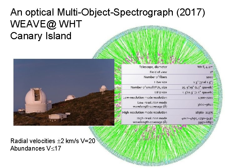
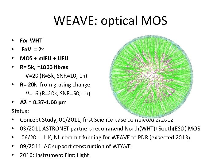
An optical Multi-Object-Spectrograph (2017) WEAVE@ WHT Canary Island Radial velocities 2 km/s V=20 Abundances V 17

The Gaia Archive

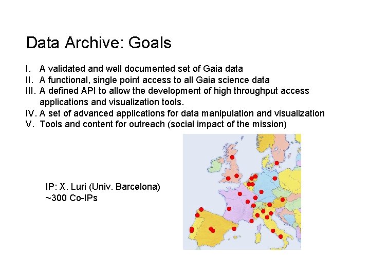
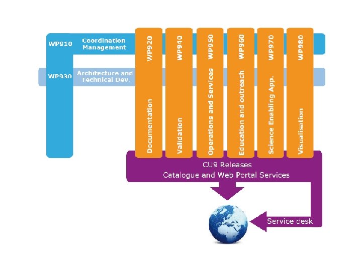
Data Archive: Goals I. A validated and well documented set of Gaia data II. A functional, single point access to all Gaia science data III. A defined API to allow the development of high throughput access applications and visualization tools. IV. A set of advanced applications for data manipulation and visualization V. Tools and content for outreach (social impact of the mission) IP: X. Luri (Univ. Barcelona) ~300 Co-IPs

Gaia and other (future) large surveys

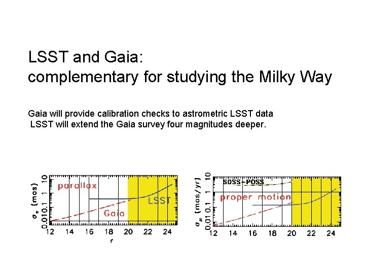
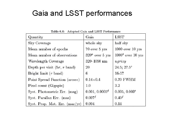
LSST and Gaia: complementary for studying the Milky Way Gaia will provide calibration checks to astrometric LSST data LSST will extend the Gaia survey four magnitudes deeper.

end

Networks and coordinated projects Scientific Exploitation: GREAT-FP 7: European Union ‘Initial Training Network (32 institutions ) REG: Red Española de Explotación Científica de Gaia (140 members, 30 institutions) GREAT-ESF: European Science Foundation (2011 -2015) (17 countries, 90 institutions) On Ground Complementary Data: GES: Gaia ESO Survey (2012 -2016) Gaia Data Achive: CU-9: Gaia DPAC (~300 participants) GENIUS-FP 7:

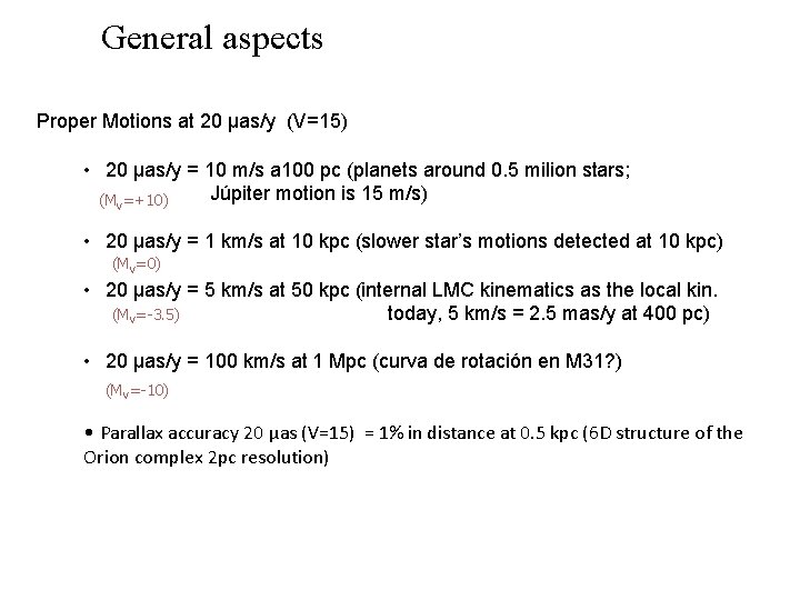
General aspects Proper Motions at 20 μas/y (V=15) • 20 μas/y = 10 m/s a 100 pc (planets around 0. 5 milion stars; Júpiter motion is 15 m/s) (MV=+10) • 20 μas/y = 1 km/s at 10 kpc (slower star’s motions detected at 10 kpc) (MV=0) • 20 μas/y = 5 km/s at 50 kpc (internal LMC kinematics as the local kin. (MV=-3. 5) today, 5 km/s = 2. 5 mas/y at 400 pc) • 20 μas/y = 100 km/s at 1 Mpc (curva de rotación en M 31? ) (MV=-10) • Parallax accuracy 20 μas (V=15) = 1% in distance at 0. 5 kpc (6 D structure of the Orion complex 2 pc resolution)

Can Gaia discover Earth Trojan? Fossils: Solar system formation Oct-2010: 1 st discov. 2010 TK 7 Difficult from Earth: Rather close to the Sun Very dispersed on sky Probability of existence of Earth trojans on stable orbits (Earth at longitude =0), Todd et al. 2011

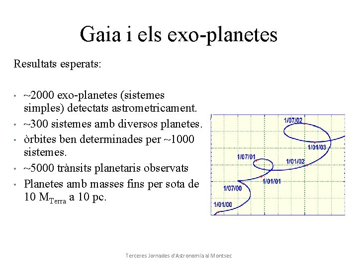
Gaia i els exo-planetes Resultats esperats: • • • ~2000 exo-planetes (sistemes simples) detectats astrometricament. ~300 sistemes amb diversos planetes. òrbites ben determinades per ~1000 sistemes. ~5000 trànsits planetaris observats Planetes amb masses fins per sota de 10 MTerra a 10 pc. Terceres Jornades d'Astronomia al Montsec

Gaia capabilities / products • Positions, proper motions and parallaxes for 1 billion stars (G < 20) • Low resolution spectrophotometry for 1 billion stars, allowing estimations of Teff, logg, Av and [Fe/H] • Radial velocities for 150 million stars (G < 16) • Atmospheric parameters, reddening and rotational velocities for 5 million stars (G < 12) • Detailed chemical abundances for 2 million stars (G < 11)

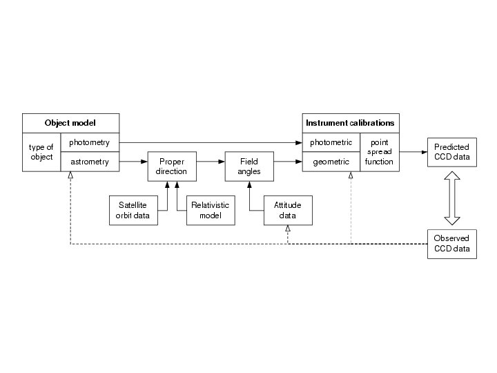
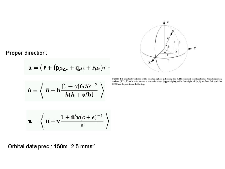
Proper direction: Orbital data prec. : 150 m, 2. 5 mms-1

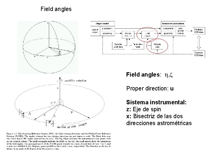
Field angles: , Proper direction: u Sistema instrumental: z: Eje de spin x: Bisectriz de las dos direcciones astrométricas

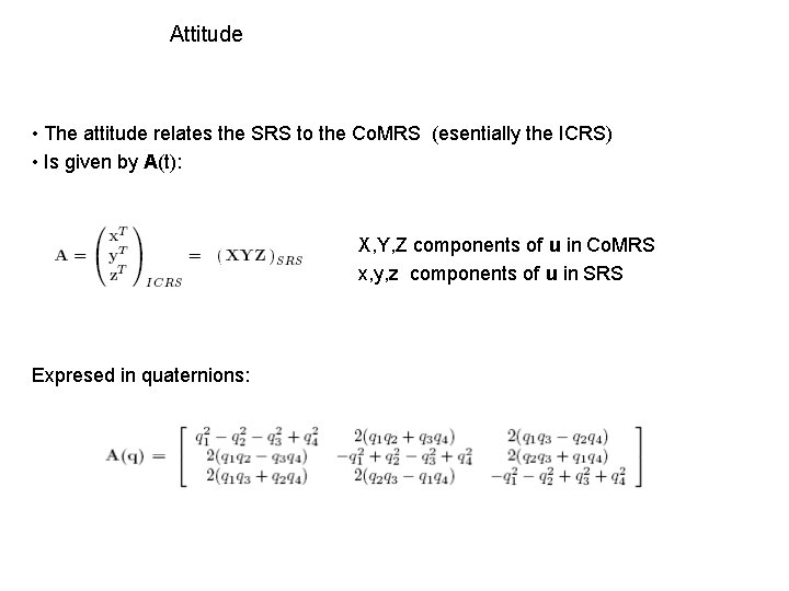
Attitude • The attitude relates the SRS to the Co. MRS (esentially the ICRS) • Is given by A(t): X, Y, Z components of u in Co. MRS x, y, z components of u in SRS Expresed in quaternions:

Instrumental calibration - (in, x, y), (in, x, y) Each CCD photometrically defined - bias, flatfield, etc. in=0, 1 x, y: position on the focal plane PSF, LSF calib. Each CCD row calibrated geometrically

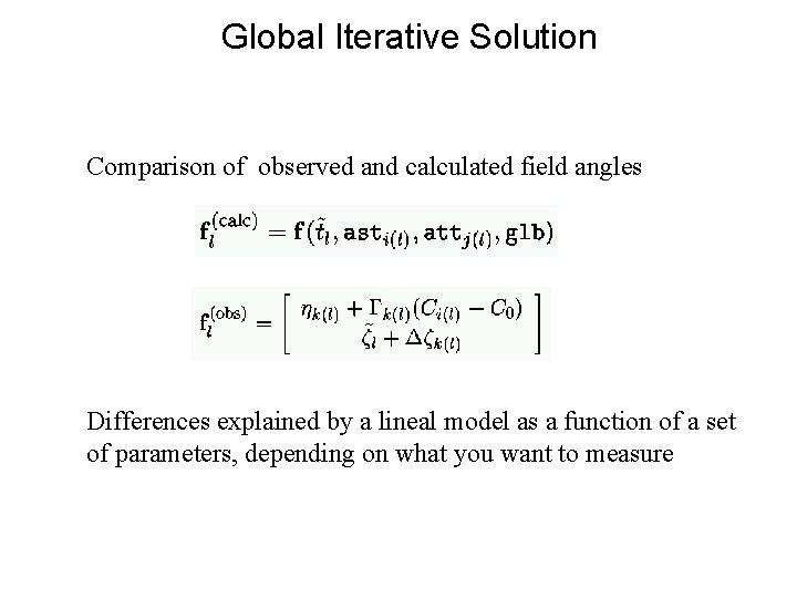
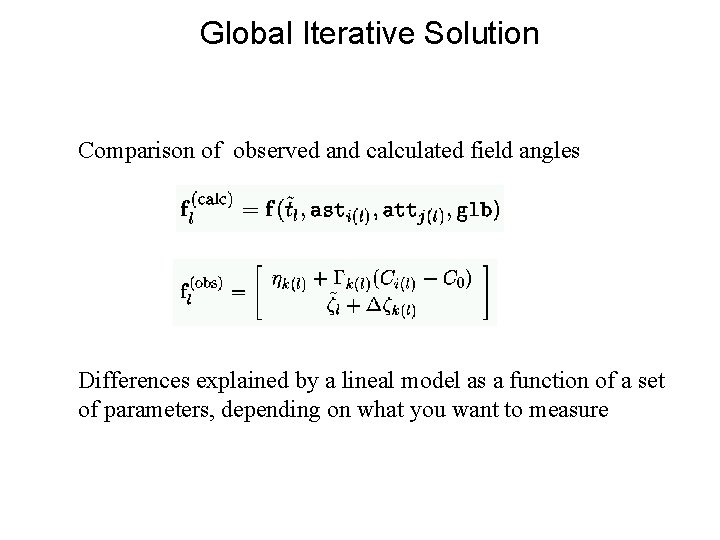
Global Iterative Solution Comparison of observed and calculated field angles Differences explained by a lineal model as a function of a set of parameters, depending on what you want to measure

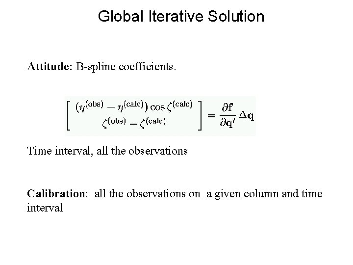
Global Iterative Solution Attitude: B-spline coefficients. Time interval, all the observations Calibration: all the observations on a given column and time interval

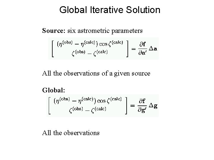
Global Iterative Solution Source: six astrometric parameters All the observations of a given source Global: All the observations

Global Iterative Solution Source: six astrometric parameters All the observations of a given source Global: All the observations

Data reduction • 1012 Individual measurements (transits) • 1010 Unknowns (all related, simultaneous determination) • 5· 109 stars(pos, pm, par) • 1. 5· 108 attitude • 10 - 50 106 calibration • Some tens of “global” • Requirements at 20 μas level (10 -10 rad) • Colours are needed for PSF, LSF (centroiding) • Radial velocities enter in astrometric model • relativistic model (orbit, ephemerides, time) • Data Volume ~500 TB – 1 PB for 5 years, 1020 -21 flop • CPU time: 1 sec/star – 30 years

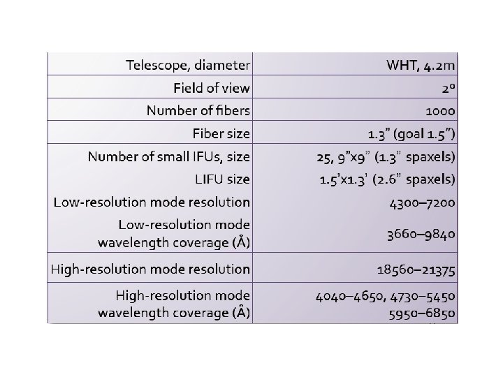
WEAVE: optical MOS • For WHT • Fo. V = 2 o • MOS + m. IFU + LIFU • R= 5 k, ~1000 fibres V=20 (R=5 k, SNR=10, 1 h) • R= 20 k from grating change V=16 (R=20 k, SNR=50, 1 h) • = 0. 37 -1. 00 μm Status: • Concept Study, 01/2011, first Science Case completed 2/2012 • 03/2011 ASTRONET partners recommend North(WHT)+South(ESO) MOS • 06/2011 UK, NL commit funding for WEAVE to PDR (expected 2013) • 09/2011 IAC support construction of WEAVE • 2016: Instrument First Light

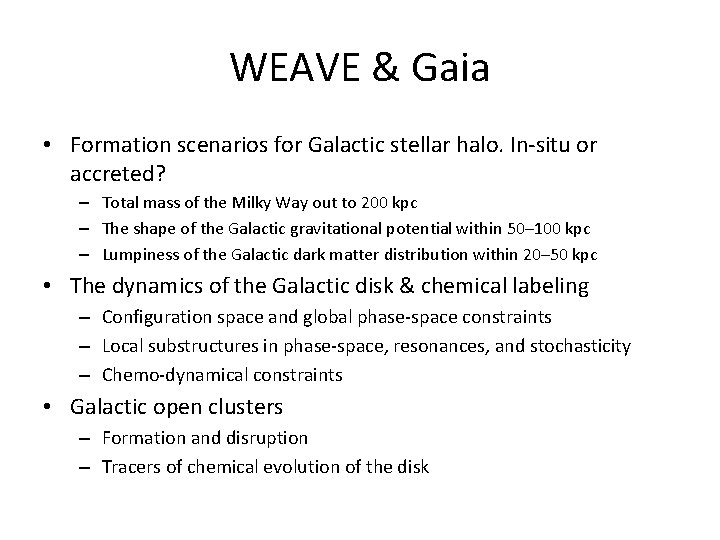
WEAVE & Gaia • Formation scenarios for Galactic stellar halo. In-situ or accreted? – Total mass of the Milky Way out to 200 kpc – The shape of the Galactic gravitational potential within 50– 100 kpc – Lumpiness of the Galactic dark matter distribution within 20– 50 kpc • The dynamics of the Galactic disk & chemical labeling – Configuration space and global phase-space constraints – Local substructures in phase-space, resonances, and stochasticity – Chemo-dynamical constraints • Galactic open clusters – Formation and disruption – Tracers of chemical evolution of the disk

Gaia and LSST performances

Field angles: , Ellipse: instantaneous scan great-circle Rectangles: the two Gaia Fo. V (BAM = 106. 5º) Sun: always 45º from the positive z axis

Global Iterative Solution Comparison of observed and calculated field angles Differences explained by a lineal model as a function of a set of parameters, depending on what you want to measure

Astrometric Global Iterative Solution

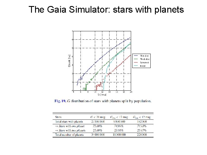
The Gaia Simulator: stars with planets

The Gaia simulator: extragalactic objects Stars per square-deg (log 10)

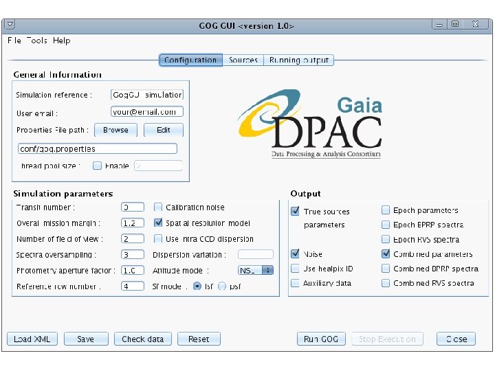
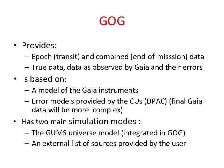
GOG • Provides: – Epoch (transit) and combined (end-of-misssion) data – True data, data as observed by Gaia and their errors • Is based on: – A model of the Gaia instruments – Error models provided by the CUs (DPAC) (final Gaia data will be more complex) • Has two main simulation modes : – The GUMS universe model (integrated in GOG) – An external list of sources provided by the user

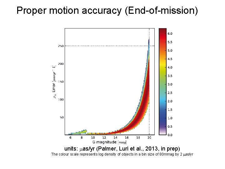
Proper motion accuracy (End-of-mission) units: as/yr (Palmer, Luri et al. , 2013, in prep) The colour scale represents log density of objects in a bin size of 80 mmag by 2 as/yr

R 136, the star cluster in the Tarantula (30 Doradus) Gaia (GIBIS) HST de Bruijne and de Marchi, 2011

QSO Detection SVM (Super Vector Machine) using BP/RP and astrometry QSO with emission-line EWs less than 5000Å removed (they are confused with cool highly reddened stars) Està al revés?

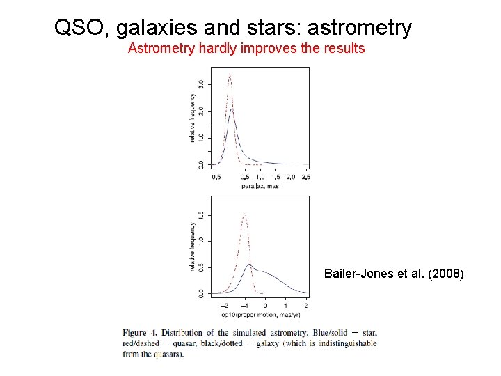
QSO, galaxies and stars: astrometry Astrometry hardly improves the results Bailer-Jones et al. (2008)

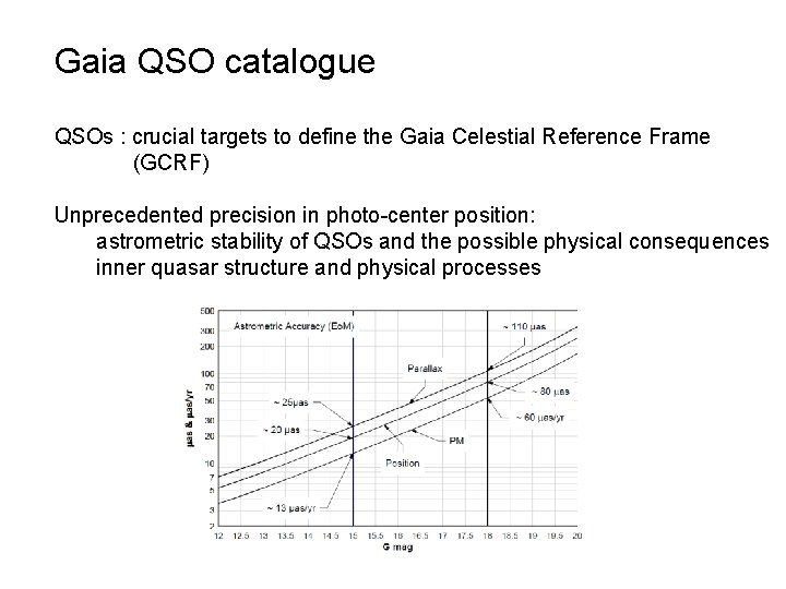
Gaia QSO catalogue QSOs : crucial targets to define the Gaia Celestial Reference Frame (GCRF) Unprecedented precision in photo-center position: astrometric stability of QSOs and the possible physical consequences inner quasar structure and physical processes

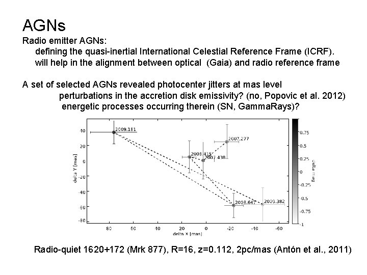
AGNs Radio emitter AGNs: defining the quasi-inertial International Celestial Reference Frame (ICRF). will help in the alignment between optical (Gaia) and radio reference frame A set of selected AGNs revealed photocenter jitters at mas level perturbations in the accretion disk emissivity? (no, Popovic et al. 2012) energetic processes occurring therein (SN, Gamma. Rays)? Radio-quiet 1620+172 (Mrk 877), R=16, z=0. 112, 2 pc/mas (Antón et al. , 2011)

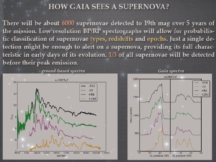
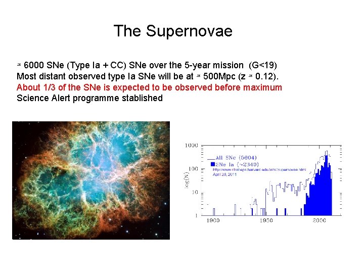
The Supernovae ≃ 6000 SNe (Type Ia + CC) SNe over the 5 -year mission (G<19) Most distant observed type Ia SNe will be at ≃ 500 Mpc (z ≃ 0. 12). About 1/3 of the SNe is expected to be observed before maximum Science Alert programme stablished

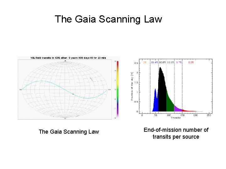
The Gaia Scanning Law End-of-mission number of transits per source

Microlensing events during the Gaia mission

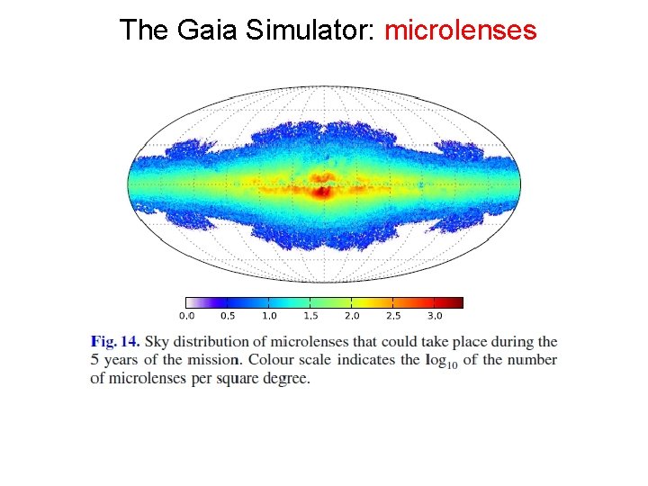
The Gaia Simulator: microlenses

Prediction of astrometric microlensing events during the Gaia mission 43 astrometric microlensing effect during the Gaia mission. The effect allows a precise measurement of the mass of a single star that is acting as a lens The 2 events that should be observable with Gaia are plotted as green squares