Two Sample Hypothesis Testing for Means from Independent

Two Sample Hypothesis Testing for Means from Independent Groups © 2010 Pearson Prentice Hall. All rights reserved

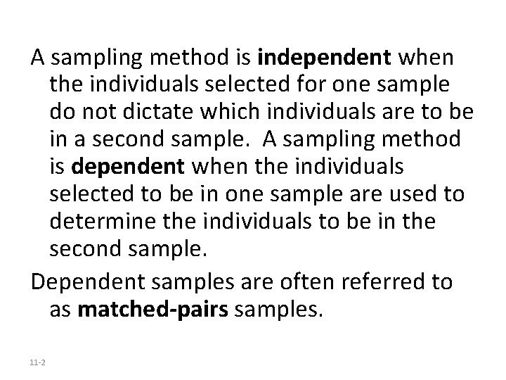
A sampling method is independent when the individuals selected for one sample do not dictate which individuals are to be in a second sample. A sampling method is dependent when the individuals selected to be in one sample are used to determine the individuals to be in the second sample. Dependent samples are often referred to as matched-pairs samples. 11 -2

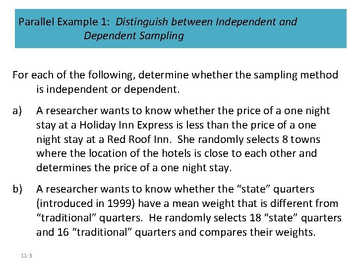
Parallel Example 1: Distinguish between Independent and Dependent Sampling For each of the following, determine whether the sampling method is independent or dependent. a) A researcher wants to know whether the price of a one night stay at a Holiday Inn Express is less than the price of a one night stay at a Red Roof Inn. She randomly selects 8 towns where the location of the hotels is close to each other and determines the price of a one night stay. b) A researcher wants to know whether the “state” quarters (introduced in 1999) have a mean weight that is different from “traditional” quarters. He randomly selects 18 “state” quarters and 16 “traditional” quarters and compares their weights. 11 -3

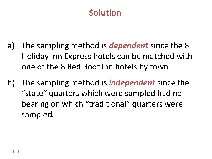
Solution a) The sampling method is dependent since the 8 Holiday Inn Express hotels can be matched with one of the 8 Red Roof Inn hotels by town. b) The sampling method is independent since the “state” quarters which were sampled had no bearing on which “traditional” quarters were sampled. 11 -4

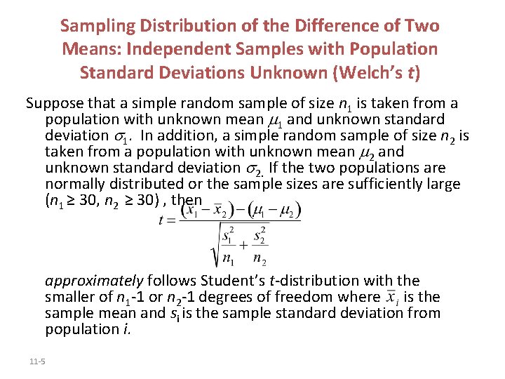
Sampling Distribution of the Difference of Two Means: Independent Samples with Population Standard Deviations Unknown (Welch’s t) Suppose that a simple random sample of size n 1 is taken from a population with unknown mean 1 and unknown standard deviation 1. In addition, a simple random sample of size n 2 is taken from a population with unknown mean 2 and unknown standard deviation 2. If the two populations are normally distributed or the sample sizes are sufficiently large (n 1 ≥ 30, n 2 ≥ 30) , then approximately follows Student’s t-distribution with the smaller of n 1 -1 or n 2 -1 degrees of freedom where is the sample mean and si is the sample standard deviation from population i. 11 -5

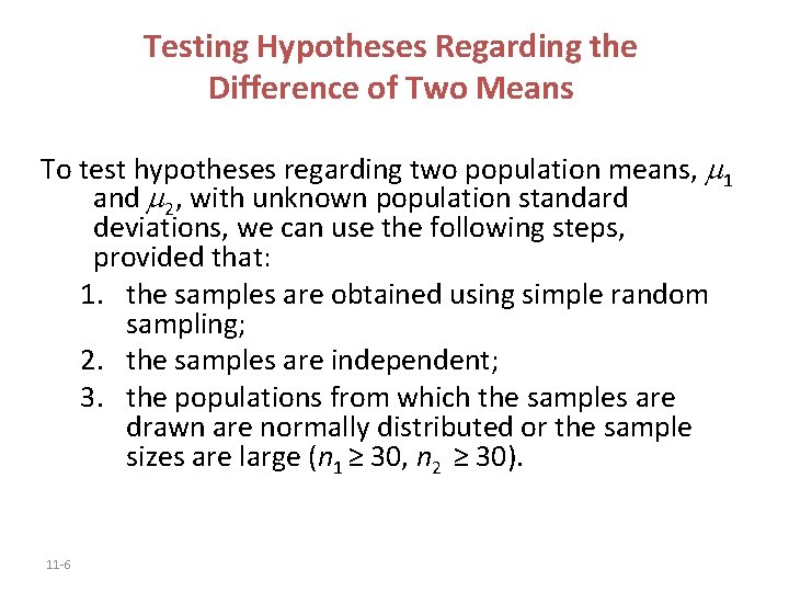
Testing Hypotheses Regarding the Difference of Two Means To test hypotheses regarding two population means, 1 and 2, with unknown population standard deviations, we can use the following steps, provided that: 1. the samples are obtained using simple random sampling; 2. the samples are independent; 3. the populations from which the samples are drawn are normally distributed or the sample sizes are large (n 1 ≥ 30, n 2 ≥ 30). 11 -6

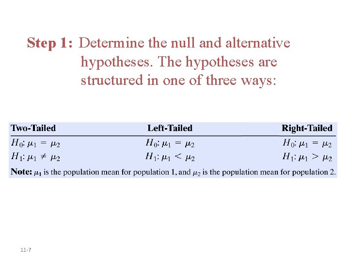
Step 1: Determine the null and alternative hypotheses. The hypotheses are structured in one of three ways: 11 -7

Step 2: Select a level of significance, , based on the seriousness of making a Type I error. 11 -8

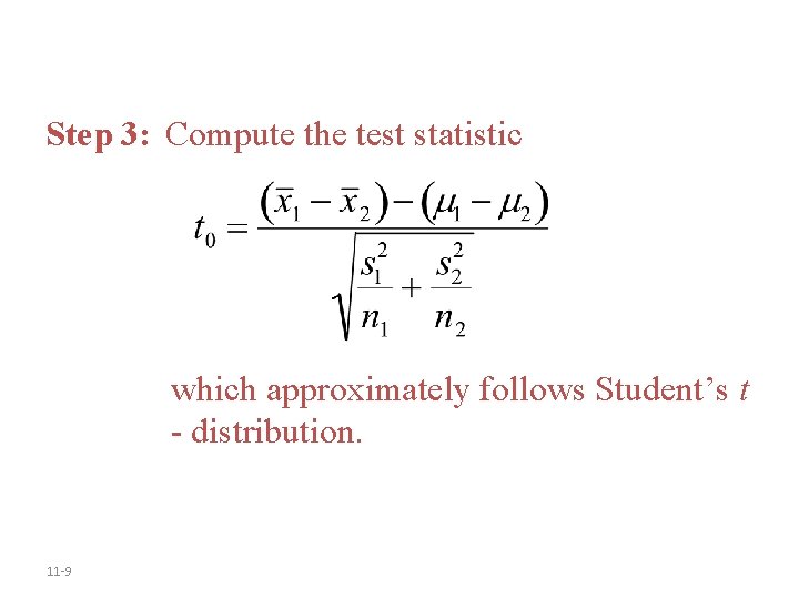
Step 3: Compute the test statistic which approximately follows Student’s t - distribution. 11 -9

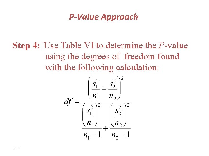
P-Value Approach Step 4: Use Table VI to determine the P-value using the degrees of freedom found with the following calculation: 11 -10

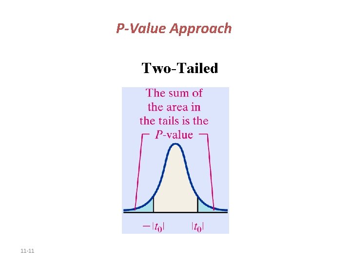
P-Value Approach Two-Tailed 11 -11

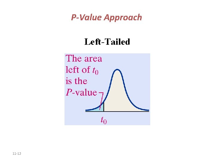
P-Value Approach Left-Tailed 11 -12

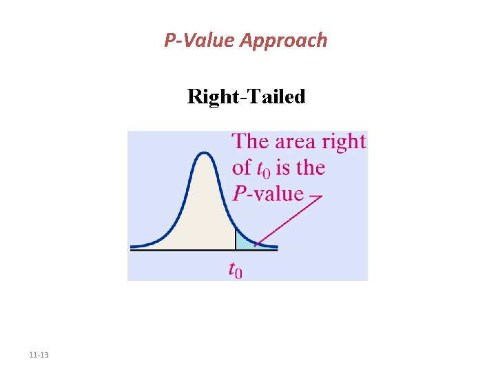
P-Value Approach Right-Tailed 11 -13

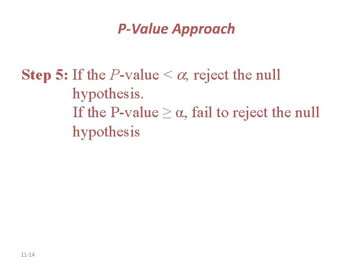
P-Value Approach Step 5: If the P-value < , reject the null hypothesis. If the P-value ≥ α, fail to reject the null hypothesis 11 -14

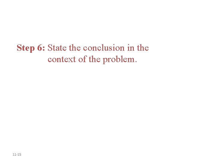
Step 6: State the conclusion in the context of the problem. 11 -15

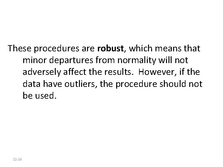
These procedures are robust, which means that minor departures from normality will not adversely affect the results. However, if the data have outliers, the procedure should not be used. 11 -16

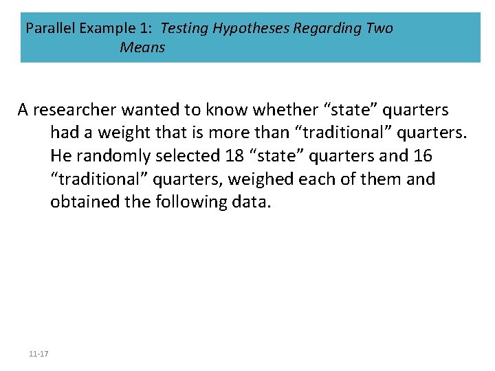
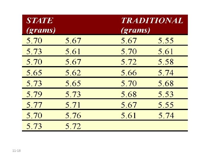
Parallel Example 1: Testing Hypotheses Regarding Two Means A researcher wanted to know whether “state” quarters had a weight that is more than “traditional” quarters. He randomly selected 18 “state” quarters and 16 “traditional” quarters, weighed each of them and obtained the following data. 11 -17

11 -18

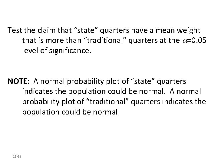
Test the claim that “state” quarters have a mean weight that is more than “traditional” quarters at the =0. 05 level of significance. NOTE: A normal probability plot of “state” quarters indicates the population could be normal. A normal probability plot of “traditional” quarters indicates the population could be normal 11 -19

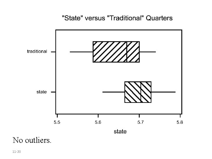
No outliers. 11 -20

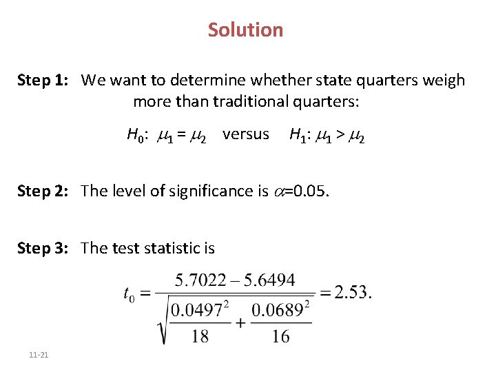
Solution Step 1: We want to determine whether state quarters weigh more than traditional quarters: H 0: 1 = 2 versus H 1 : 1 > 2 Step 2: The level of significance is =0. 05. Step 3: The test statistic is 11 -21

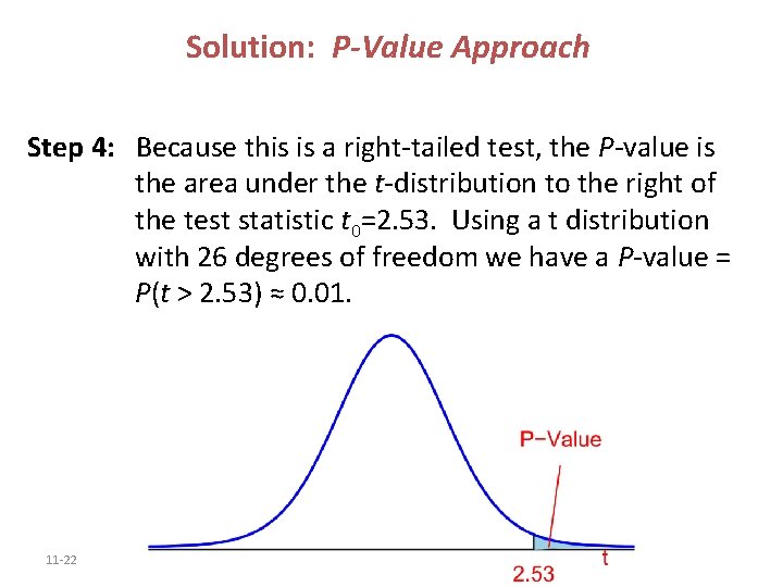
Solution: P-Value Approach Step 4: Because this is a right-tailed test, the P-value is the area under the t-distribution to the right of the test statistic t 0=2. 53. Using a t distribution with 26 degrees of freedom we have a P-value = P(t > 2. 53) ≈ 0. 01. 11 -22

Solution: P-Value Approach Step 5: Since the P-value is less than the level of significance =0. 05, we reject the null hypothesis. 11 -23

Solution Step 6: There is sufficient evidence at the =0. 05 level to conclude that the state quarters weigh more than the traditional quarters. 11 -24

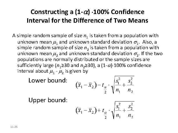
Constructing a (1 - ) 100% Confidence Interval for the Difference of Two Means A simple random sample of size n 1 is taken from a population with unknown mean 1 and unknown standard deviation 1. Also, a simple random sample of size n 2 is taken from a population with unknown mean 2 and unknown standard deviation 2. If the two populations are normally distributed or the sample sizes are sufficiently large (n 1≥ 30 and n 2≥ 30), a (1 - ) 100% confidence interval about 1 - 2 is given by Lower bound: Upper bound: 11 -25

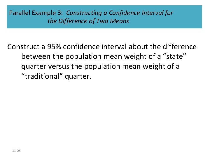
Parallel Example 3: Constructing a Confidence Interval for the Difference of Two Means Construct a 95% confidence interval about the difference between the population mean weight of a “state” quarter versus the population mean weight of a “traditional” quarter. 11 -26

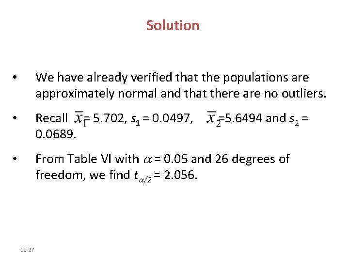
Solution • We have already verified that the populations are approximately normal and that there are no outliers. • Recall = 5. 702, s 1 = 0. 0497, 0. 0689. • From Table VI with = 0. 05 and 26 degrees of freedom, we find t /2 = 2. 056. 11 -27 =5. 6494 and s 2 =

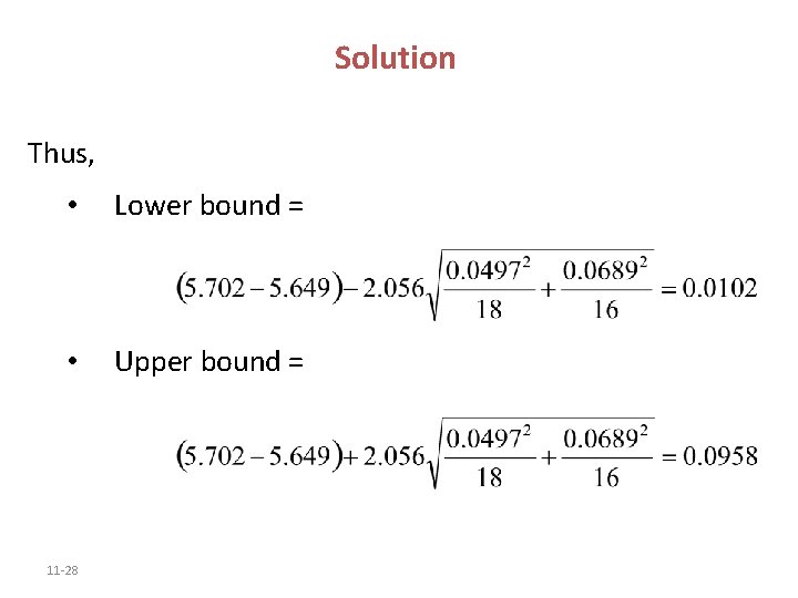
Solution Thus, • Lower bound = • Upper bound = 11 -28

Solution We are 95% confident that the mean weight of the “state” quarters is between 0. 0102 and 0. 0958 ounces more than the mean weight of the “traditional” quarters. Since the confidence interval does not contain 0, we conclude that the “state” quarters weigh more than the “traditional” quarters. 11 -29