Hypothesis Testing Hypothesis testing is an inferential process

Hypothesis Testing • Hypothesis testing is an inferential process • Using limited information to reach a general conclusion • Observable evidence from the sample data • Unobservable fact about the population • Formulate a specific, testable research hypothesis about the population

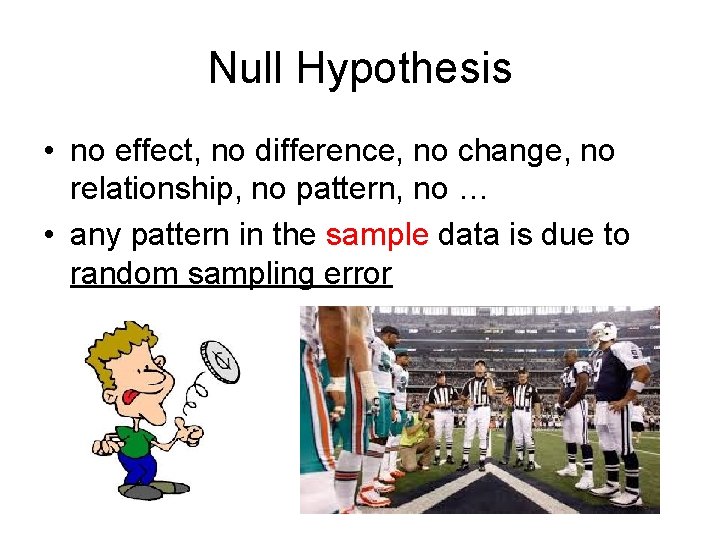
Null Hypothesis • no effect, no difference, no change, no relationship, no pattern, no … • any pattern in the sample data is due to random sampling error

Type I Error • A researcher finds evidence for a significant result when, in fact, there is no effect (no relationship) in the population. • The researcher has, by chance, selected an extreme sample that appears to show the existence of an effect when there is none. • The p-value identifies the probability of a Type I error.

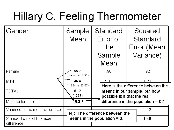
Significance in Comparisons • The key to becoming confident in a sample mean is determining the standard error of the mean. • But if research was simply about becoming confident in and reporting our confidence in a sample mean, research would not be all that interesting.

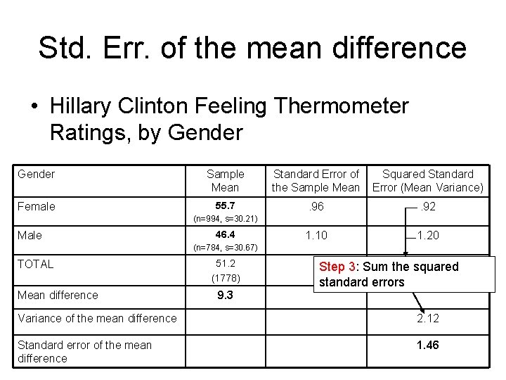
Hillary C. Feeling Thermometer Gender Female Sample Standard Squared Mean Error of Standard the Error (Mean Sample Variance) Mean 55. 7 . 96 . 92 1. 10 1. 20 (n=994, s=30. 21) Male 46. 4 (n=784, s=30. 67) TOTAL Mean difference Variance of the mean difference Standard error of the mean difference 51. 2 (1778) 9. 3 Here is the difference between the means in our sample, but how possible is it that the real difference in the population = 0? H 0: The difference between the means in the population = 0. 2. 12 1. 46

Significance in Comparisons • The key to figuring out whether the difference between two means is significant (different from 0 in the population), we need to calculate the standard error of the mean difference.

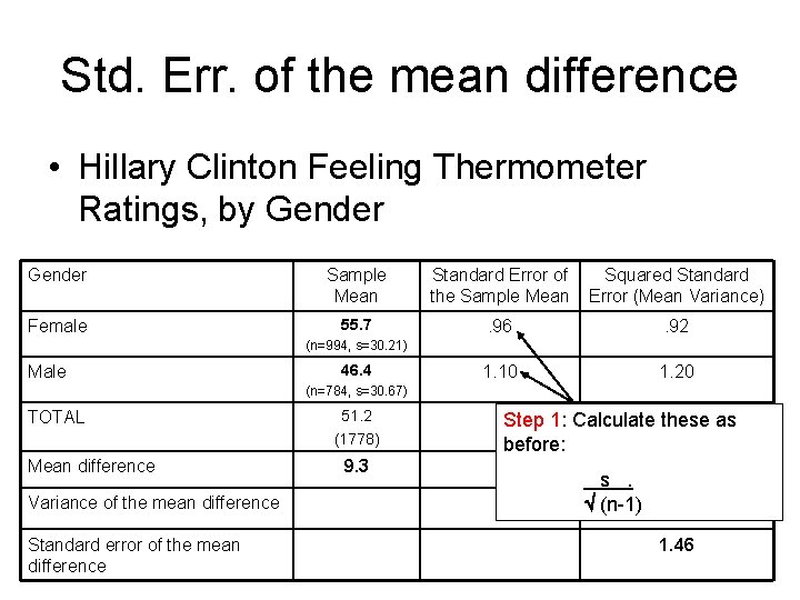
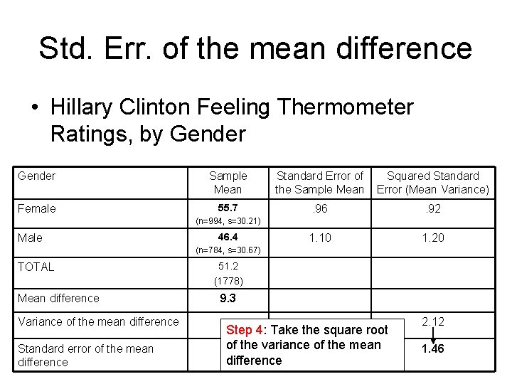
Std. Err. of the mean difference • Hillary Clinton Feeling Thermometer Ratings, by Gender Sample Mean Standard Error of the Sample Mean Squared Standard Error (Mean Variance) Female 55. 7 . 96 . 92 1. 10 1. 20 (n=994, s=30. 21) Male 46. 4 (n=784, s=30. 67) TOTAL Mean difference Variance of the mean difference Standard error of the mean difference 51. 2 (1778) 9. 3 Step 1: Calculate these as before: s. Ö (n-1) 2. 12 1. 46

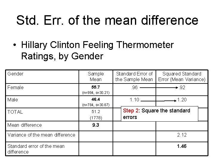
Std. Err. of the mean difference • Hillary Clinton Feeling Thermometer Ratings, by Gender Sample Mean Standard Error of the Sample Mean Squared Standard Error (Mean Variance) Female 55. 7 . 96 . 92 1. 10 1. 20 (n=994, s=30. 21) Male 46. 4 (n=784, s=30. 67) TOTAL Mean difference 51. 2 (1778) Step 2: Square the standard errors 9. 3 Variance of the mean difference 2. 12 Standard error of the mean difference 1. 46

Std. Err. of the mean difference • Hillary Clinton Feeling Thermometer Ratings, by Gender Sample Mean Standard Error of the Sample Mean Squared Standard Error (Mean Variance) Female 55. 7 . 96 . 92 1. 10 1. 20 (n=994, s=30. 21) Male 46. 4 (n=784, s=30. 67) TOTAL Mean difference 51. 2 (1778) Step 3: Sum the squared standard errors 9. 3 Variance of the mean difference 2. 12 Standard error of the mean difference 1. 46

Std. Err. of the mean difference • Hillary Clinton Feeling Thermometer Ratings, by Gender Sample Mean Standard Error of the Sample Mean Squared Standard Error (Mean Variance) Female 55. 7 . 96 . 92 1. 10 1. 20 (n=994, s=30. 21) Male 46. 4 (n=784, s=30. 67) TOTAL Mean difference Variance of the mean difference Standard error of the mean difference 51. 2 (1778) 9. 3 Step 4: Take the square root of the variance of the mean difference 2. 12 1. 46

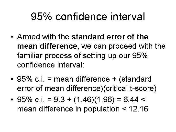
95% confidence interval • Armed with the standard error of the mean difference, we can proceed with the familiar process of setting up our 95% confidence interval: • 95% c. i. = mean difference + (standard error of mean difference)(critical t-score) • 95% c. i. = 9. 3 + (1. 46)(1. 96) = 6. 44 < mean difference in population < 12. 16

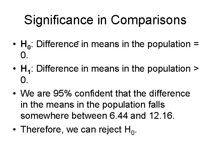
Significance in Comparisons • H 0: Difference in means in the population = 0. • H 1: Difference in means in the population > 0. • We are 95% confident that the difference in the means in the population falls somewhere between 6. 44 and 12. 16. • Therefore, we can reject H 0.

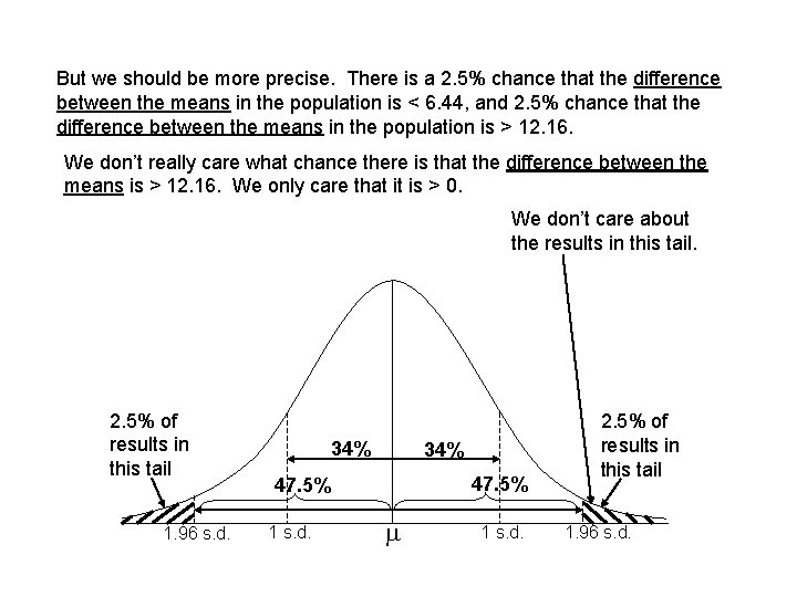
But we should be more precise. There is a 2. 5% chance that the difference between the means in the population is < 6. 44, and 2. 5% chance that the difference between the means in the population is > 12. 16. We don’t really care what chance there is that the difference between the means is > 12. 16. We only care that it is > 0. We don’t care about the results in this tail. 2. 5% of results in this tail 1. 96 s. d. 34% 47. 5% 1 s. d. m 1 s. d. 2. 5% of results in this tail 1. 96 s. d.

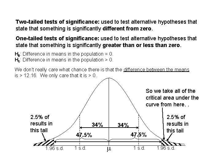
Two-tailed tests of significance: used to test alternative hypotheses that state that something is significantly different from zero. One-tailed tests of significance: used to test alternative hypotheses that state that something is significantly greater than or less than zero. H 0: Difference in means in the population = 0. H 1: Difference in means in the population > 0. We don’t really care what chance there is that the difference between the means is > 12. 16. We only care that it is > 0. So we take all of the critical area under the curve from here. . 2. 5% of results in this tail 1. 96 s. d. 34% 47. 5% 1 s. d. m 1 s. d. 2. 5% of results in this tail 1. 96 s. d.

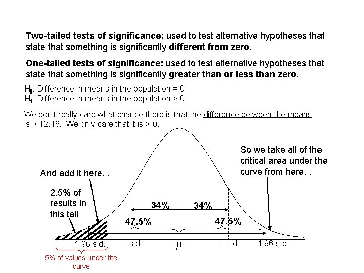
Two-tailed tests of significance: used to test alternative hypotheses that state that something is significantly different from zero. One-tailed tests of significance: used to test alternative hypotheses that state that something is significantly greater than or less than zero. H 0: Difference in means in the population = 0. H 1: Difference in means in the population > 0. We don’t really care what chance there is that the difference between the means is > 12. 16. We only care that it is > 0. So we take all of the critical area under the curve from here. . And add it here. . 2. 5% of results in this tail 1. 96 s. d. 5% of values under the curve 34% 47. 5% 1 s. d. m 1 s. d. 1. 96 s. d.

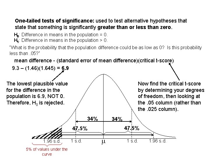
One-tailed tests of significance: used to test alternative hypotheses that state that something is significantly greater than or less than zero. H 0: Difference in means in the population = 0. H 1: Difference in means in the population > 0. “What is the probability that the population difference could be as low as 0? Is this probability less than. 05? ” mean difference - (standard error of mean difference)(critical t-score) 9. 3 – (1. 46)(1. 645) = 6. 9 The lowest plausible value for the difference in the population is 6. 9, NOT 0. Therefore, H 0 is rejected. Now find the critical t-score by determining your degrees of freedom, then looking at the. 05 column (rather than the. 025 column). 34% 47. 5% 1. 96 s. d. 5% of values under the curve 1 s. d. m 1 s. d. 1. 96 s. d.

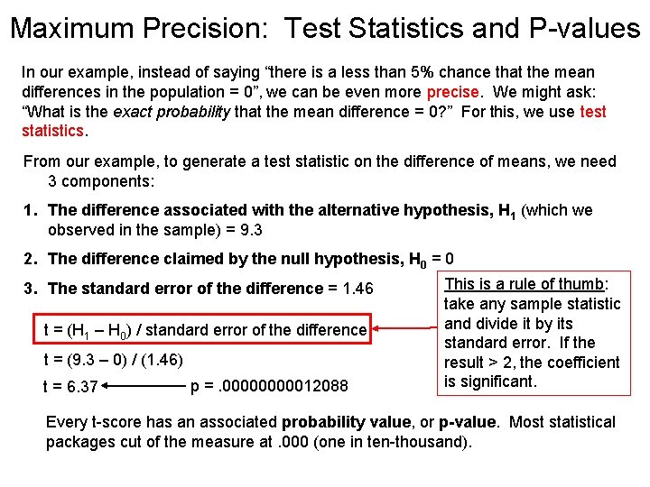
Maximum Precision: Test Statistics and P-values In our example, instead of saying “there is a less than 5% chance that the mean differences in the population = 0”, we can be even more precise. We might ask: “What is the exact probability that the mean difference = 0? ” For this, we use test statistics. From our example, to generate a test statistic on the difference of means, we need 3 components: 1. The difference associated with the alternative hypothesis, H 1 (which we observed in the sample) = 9. 3 2. The difference claimed by the null hypothesis, H 0 = 0 3. The standard error of the difference = 1. 46 t = (H 1 – H 0) / standard error of the difference t = (9. 3 – 0) / (1. 46) t = 6. 37 p =. 0000012088 This is a rule of thumb: take any sample statistic and divide it by its standard error. If the result > 2, the coefficient is significant. Every t-score has an associated probability value, or p-value. Most statistical packages cut of the measure at. 000 (one in ten-thousand).

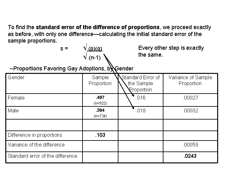
To find the standard error of the difference of proportions, we proceed exactly as before, with only one difference—calculating the initial standard error of the sample proportions. Every other step is exactly s= Ö (p)(q) the same. Ö (n-1) --Proportions Favoring Gay Adoptions, by Gender Sample Proportion Standard Error of the Sample Proportion Variance of Sample Proportion Female . 497 . 016 . 00027 . 018 . 00032 (n=922) Male . 394 (n=734) Difference in proportions . 103 Variance of the difference . 00059 Standard error of the difference . 0243