Topics in Health Economics Matilde P Machado matilde

Topics in Health Economics Matilde P. Machado matilde. machado@uc 3 m. es 1

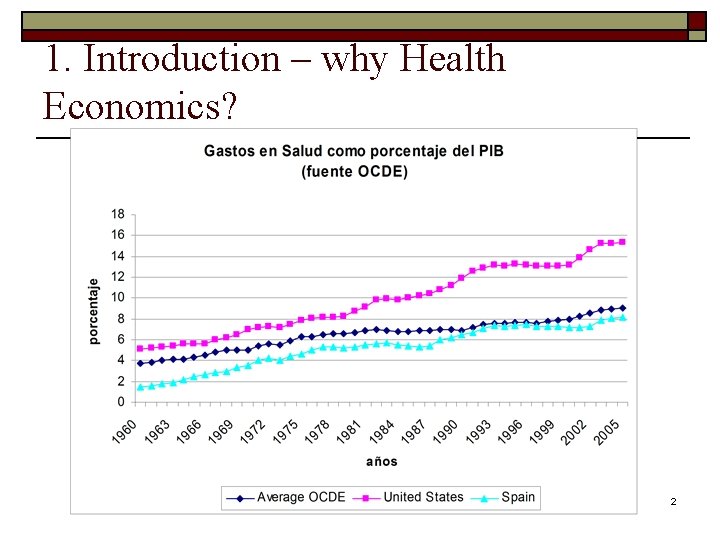
1. Introduction – why Health Economics? 2

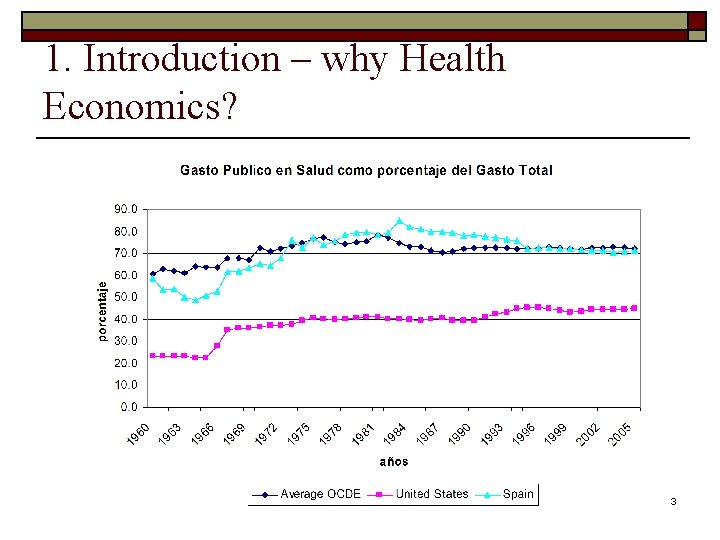
1. Introduction – why Health Economics? 3

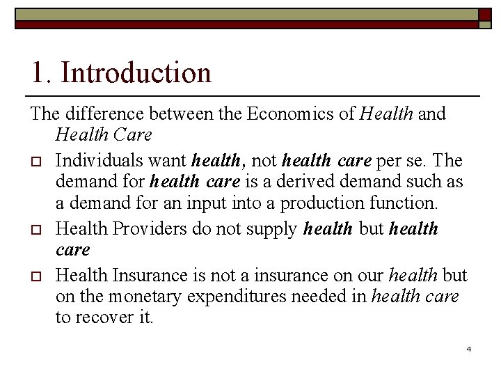
1. Introduction The difference between the Economics of Health and Health Care o Individuals want health, not health care per se. The demand for health care is a derived demand such as a demand for an input into a production function. o Health Providers do not supply health but health care o Health Insurance is not a insurance on our health but on the monetary expenditures needed in health care to recover it. 4

1. Introduction q. Course is on the Economics of health care, i. e. we are going to talk about Demand Supply of health care services. q. Health Economics is also about health, for example, estimation of health production functions (where there are other inputs besides health care). q. Reading: Arrow, K. (1963). “Uncertainty and the Welfare Economics of Medical Care, ” AER (1963), 5, 941 -973. 5

1. Introduction Arrow (1963) – Summary: q. Examines in which ways the medical care market diverges from the competitive benchmark q. Argues that all special features emerge due to uncertainty. q q Uncertainty from the demand side: occurrence of the disease Uncertainty from the supply side: treatment results q. Argues society creates institutions to palliate the nonoptimalities which do not allow competition to emerge. 6

1. Introduction Arrow (1963) Special Characteristics of the Medical Care market: q. Demand Side: q q. Supply q The nature of demand: irregular and unpredictable. Moreover the risks involved may be very costly in terms of utility (including death) side: Expected behavior of suppliers: q q q Asymmetry of Information (the doctor has more information): Often we are looking for diagnosis when visiting the doctor/hospital, we cannot, therefore, judge the quality of the service since the service is information. Although, they could use this informational advantage in their favor, we do not expect physicians and hospitals to behave as salesmen, we expect them to have our interest in mind. The reason may lie in the fact that most relations between physicians and patients are long-term. The ideal way to pay providers would be dependent on the outcome. As this is not possible, usually people establish long-term relationship with their physicians that translates in “good” incentives. Most people, believe that individuals should have access to (some/all) health care irrespectively of their capability to pay for it. 7

1. Introduction Arrow (1963) q. Supply q q q side (cont): Product Uncertainty: regarding most adequate treatment, treatment prospects, side-effects, etc. , which can be very costly in terms of utility. Again the doctor has more information. Due to the uncertainty regarding treatment results, the medical care market responded with rigid entry requirements that reduce the uncertainty among patients about the quality of the services provided. Supply conditions: Entry is regulated by licensing – the purpose is to guarantee minimal quality, but isn’t it too strict? There is a tough selection in entry and finishing medicine school as well as training practices enough, in Spain also the MIR. Why shouldn’t other e. g. nurses be able to perform some of the known “medical practice? ” Pricing: extensive price discrimination by income (individual doctors). Nowadays, we find many different pricing schedules depending on the insurers agreements. 8

1. Introduction Arrow (1963) Problems of Insurance (besides the impossibility of getting insurance on several risks): 1. Moral Hazard – insurance is welfare improving: the individual is risk averse and is willing to pay a premium and insurance agencies by pooling risks are able to profit. However, this is true when the “loss” is exogenous. However, when individuals take up insurance does that affect the “loss” ? And in that case is insurance profitable? Questions: Does an individual with total coverage by health insurance go more to the doctor than the same individual without health insurance? Has insurance had an effect on his decisions? And incentives (for example the incentive to look for the best price)? 9

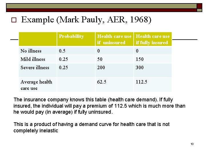
o Example (Mark Pauly, AER, 1968) Probability Health care use if uninsured if fully insured No illness 0. 5 0 0 Mild illness 0. 25 50 150 Severe illness 0. 25 200 300 62. 5 112. 5 Average health care use The insurance company knows this table (health care demand). If fully insured, the individual will pay a premium of 112. 5 which is much more than he would pay (in average) if fully uninsured. This is a product of having a demand curve for health care that is not completely inelastic 10

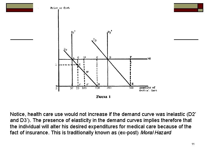
Notice, health care use would not increase if the demand curve was inelastic (D 2’ and D 3’). The presence of elasticity in the demand curves implies therefore that the individual will alter his desired expenditures for medical care because of the fact of insurance. This is traditionally known as (ex-post) Moral Hazard 11

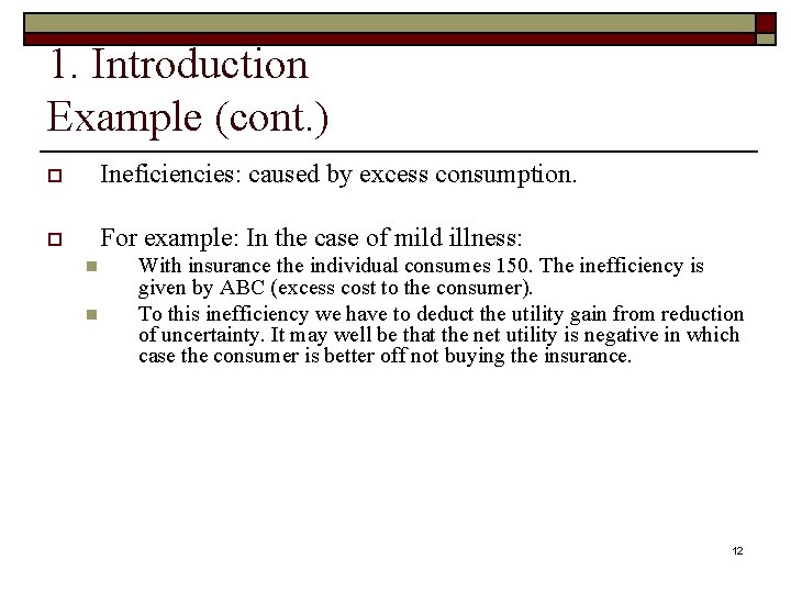
1. Introduction Example (cont. ) o Ineficiencies: caused by excess consumption. o For example: In the case of mild illness: n n With insurance the individual consumes 150. The inefficiency is given by ABC (excess cost to the consumer). To this inefficiency we have to deduct the utility gain from reduction of uncertainty. It may well be that the net utility is negative in which case the consumer is better off not buying the insurance. 12

1. Introduction Arrow (1963) Some Actions to limit Moral Hazard o Because of Moral Hazard, co-payments (and co-insurance) have been introduced. Are they effective in controlling moral hazard? o Also are doctors prescriptions and procedures different for individuals with and without insurance? Are all services in medical care the same? (e. g. typically surgery is considered Moral Hazard free or close to it). To control for moral hazard from physicians, the so called HMOs (Health Maintenance Organizations) emerged. In the HMOs the insurer controls the provider of medical services and thereby controls the costs (quantity as well as prices of the service delivered). 13

1. Introduction Arrow (1963) 2. Adverse Selection – he does not discuss this. We will see this later. 14

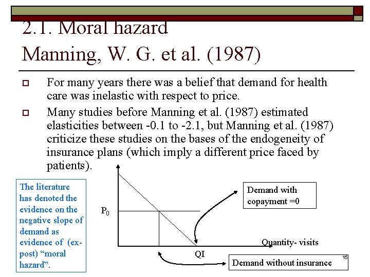
2. 1. Moral hazard Manning, W. G. et al. (1987) o o For many years there was a belief that demand for health care was inelastic with respect to price. Many studies before Manning et al. (1987) estimated elasticities between -0. 1 to -2. 1, but Manning et al. (1987) criticize these studies on the bases of the endogeneity of insurance plans (which imply a different price faced by patients). The literature has denoted the evidence on the negative slope of demand as evidence of (expost) “moral hazard”. Demand with copayment =0 P 0 Quantity- visits QI Demand without insurance 15

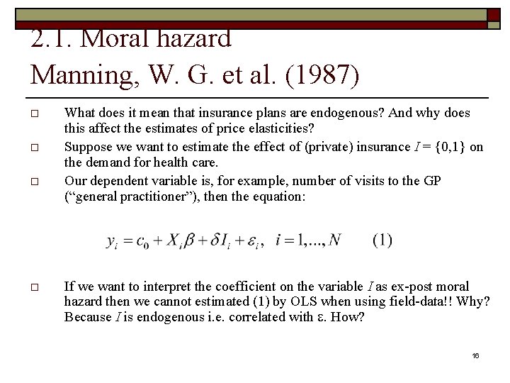
2. 1. Moral hazard Manning, W. G. et al. (1987) o o What does it mean that insurance plans are endogenous? And why does this affect the estimates of price elasticities? Suppose we want to estimate the effect of (private) insurance I = {0, 1} on the demand for health care. Our dependent variable is, for example, number of visits to the GP (“general practitioner”), then the equation: If we want to interpret the coefficient on the variable I as ex-post moral hazard then we cannot estimated (1) by OLS when using field-data!! Why? Because I is endogenous i. e. correlated with e. How? 16

2. 1. Moral hazard Manning, W. G. et al. (1987) o o o Suppose that are unobservably sicker people are more likely to contract the insurance (Adverse selection), then I and e are positively correlated. This implies that if we estimate (1) with OLS, has a positive bias. Suppose that those that are more risk averse (i. e. that conditional on health go more to the doctor) are the ones that decide to take the insurance. Risk aversion is not an observable characteristic and therefore we would be overestimating the effect of the insurance or underestimating in the case that risk-aversers take better care of their health in general. It could also be that once an individual has insurance he substitutes “home” health care by medical health care in which case the individual may need more visits (Ex-ante Moral Hazard). In this case we would overestimate the effect of the insurance. Suppose those with unobservably (to us) worse health are denied insurance (Risk Selection) which is the opposite of Adverse Selection, then we may underestimate because I and e would be negatively correlated. Finally, imagine the doctors induce more demand from those with insurance, then would be overestimated (Supply Induced Demand). 17

2. 1. Moral hazard Manning, W. G. et al. (1987) o What can be done? n Use Instrumental variables for I – Remember: Instrumental variables have to satisfy two conditions: o o n however it is difficult to think of a variable that is strongly correlated with I while having no impact on demand for visits. One example of estimation with IV is Vera (1999) (He used variables such as social class and occupation as IVs) Use examples where Insurance is exogenous: o o n Be correlated with the endogenous variable I. Note: a weak instrument can be worse than no instrument (Bound et al. 1993)! Not correlated with e, i. e. are only correlated with y through I Randomized experiment – e. g. Manning et al. , 1987 Natural experiments – e. g. Chiappori et al. (1998), Barros, Machado, Sanzde-Galdeano (2008) Use examples where demand is inelastic (in this case the effect of insurance is pure adverse selection. o Hospitalizations, surgeries, etc – e. g. Holly et al. (1998), (2002) 18

2. 1. Moral hazard Manning, W. G. et al. (1987) o What do Manning et al. (1987) do? n n n They guarantee the exogeneity of the insurance plan by randomizing different insurance plans on a population (“Rand Health Insurance Experiment”). Once insurance is considered exogenous then the estimation of price elasticities is trivial. Their main result: the price elasticity of demand is around -0. 2 They reject the hypothesis that less coverage may increase total expenditures (through more expensive channels e. g. hospitalizations) The Rand HIE has received various criticisms but is still a reference in the literature. 19

2. 1. Moral hazard Manning, W. G. et al. (1987) The HIE: o 6 different sites o Families were randomly enrolled in different fee-for-service plans and 1 prepaid-group-practice (HMO). o The fee-for-service plans varied along 2 dimensions: n n n o o the coinsurance rate (% paid out-of-pocket) {0, 25, 50, 95} the upper limit on annual out-of-pocket expenses (Maximum Dollar Expenditure MDE) {5, 10, 15}% family income with a maximum of 1000 dollars. Expenditures beyond MDE were reimbursed in full. 2 other plans: one had 95% co-insurance+150$ MDE/person (450 per family) 70 % families enrolled for 3 years, 30% for 5 years Families were given a lump sum of money to assure noone was worse off. This was believed to minimize attrition/refusal. Still, attrition was higher at higher coinsurance rates although within a given plan they did not detect selection, i. e. those that drop out were on average similar to those that stayed in the experiment. 20

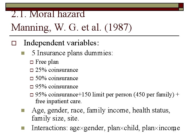
2. 1. Moral hazard Manning, W. G. et al. (1987) o Independent variables: n 5 Insurance plans dummies: o o o n n Free plan 25% coinsurance 50% coinsurance 95% coinsurance+150 limit person (450 per family) + free inpatient care. Age, gender, race, family income, health status, family size, site. Interactions: age gender, plan child, plan income 21

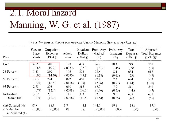
2. 1. Moral hazard Manning, W. G. et al. (1987) 22

2. 1. Moral hazard Manning, W. G. et al. (1987) Summary of results (Sample Means): 1. The p. c. expenses on the free plan are 45% higher than on the 95% coinsurance 2. Cost sharing affects primarily the number of medical contacts (versus intensity or prices) 3. The largest decrease in the use of outpatient occurs from the free plan to the 25% (visits drop 26. 8% and outpatient expenditures drop 23. 5%) 4. No statistically significant differences in the inpatient use between 25, 50, 95% coinsurance plans (perhaps due to the fact that the MED was easily reached) 23

Results of the experiment o Poor adults in the free plan improved their blood pressure over paying plans. n o o Reduction would lower mortality by 10 percent each year among this group Modest improvement in corrected vision also for poor adults Individuals in the free plan also improved the health of the gums and caries 24

2. 1. Moral hazard Manning, W. G. et al. (1987) o Data characteristics: n n n o Lots of zeros – people that never go to the doctor in a year The distribution among the users is skewed Outpatient and Inpatient users have different distribution of medical expenditures Because of these characteristics of the data they explore a 4 equation model. Simple means differences also yield consistent effects of the insurance plan (due to randomization) but they claim are very imprecise because of the characteristics of the data. Controlling for covariates allows to control for imbalances between the sites and across plans in the population characteristics but off course is parametric. 25

2. 1. Moral Hazard (Barros, P. Machado, Sanz-de-Galdeano, JHE 2008 ) o Title: Moral hazard and the demand for health services: a matching estimator approach o o Objective: To estimate the impact of extra health insurance coverage, beyond a National Health System, on the demand for several health services. We focus on the most common health insurance plan in Portugal, ADSE, which is given to all civil servants and their dependents. We argue that this insurance is exogenous, i. e. , not correlated with beneficiaries’ health status. Hence, under this identifying assumption we do not have to deal with the typical endogeneity issues of the extra (or private) insurance. 26

2. 1. Moral Hazard (Barros, P. Machado, Sanz-de-Galdeano , JHE 2008 ) o o Treatment group: ADSE beneficiaries Control Group: NHS alone The identifying assumption is that ADSE is exogenous, i. e. conditional on certain observables it is not correlated with unobserved (to us) health. Note: We discard all other individuals from the sample such as other subsistemas because the insurance coverage and copayments may differ from the rest of the control group, which may affect behavior. Also there may be non-observable variables correlated with the insurance type that may also affect individuals' behavior. 27

2. 1. Moral Hazard (Barros, P. Machado, Sanz-de-Galdeano , JHE 2008 ) o ADSE Characteristics: Agreements with private providers such that beneficiaries have small co-payments. Higher co-payment for providers outside ADSE network. ADSE beneficiaries may use NHS as any other person, subject to its small co-payments and exemptions. No GP as gate-keeper 28

2. 1. Moral Hazard (Barros, P. Machado, Sanz-de-Galdeano, JHE 2008 ) Contributions of this paper to the large literature: o o Dataset: Make use of a specific feature of the Portuguese health system whereby civil servants have exogenous additional health insurance coverage. This means 10% of observations are covered by an insurance unrelated to their health status. ► no need for IVs. Methodology: Matching estimator approach (Abadie and Imbens, 2006 a), does not impose any functional form on the impact of extra coverage on the demand allows for heterogeneous impacts Dep. Variable: We estimate the impact on several health services. Traditionally the literature uses “number of visits to the doctor (in last 3 M)” but this is a nonhomogeneous, measurement error correlated with the insurance status, subject to inducement? ADSE pays per visit. So we also use “number of blood and urine tests in last 3 M” (more homogeneous, quality independent of the insurance status, still may be subject to inducement) and “at least one visit to the dentist in last year” (hardly subject to inducement, ADSE pays per procedure). Time effect: Analysis by age group. Older individuals are subject to treatment for a longer period of time. Immediate versus cumulative effects. Suppose treatment effects are positive and accumulate over time, than older individuals may have been subject to treatment longer, this means that the difference in health from their counterpart should be larger and therefore the difference in 29 demand should be smaller, we would be underestimating moral hazard for the elderly because the ADSE would be unobservably healthier.

2. 1. Moral Hazard (Barros, P. Machado, Sanz-de-Galdeano, JHE 2008) Ø Portuguese Health Survey 1998/99. HH survey with info on: Ø Socio-demographic characteristics, income level, subjective & objective health measures, health-related habits, HI status (84% NHS only, ADSE 9. 99%). Ø Health care demand measures used: physician visits in previous 3 months, blood and urine tests in previous 3 months, at least one visit to the dentist in previous 12 months. No information where visits or tests were done in the private or public sector. Ø Sample exclusions (no Heath Insurance (HI) status, pregnant women, inconsistent answers, info provided by family member, HI different from ADSE or NHS). Total obs = 21151 to 21908 30

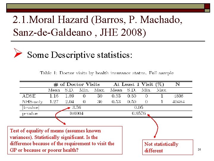
2. 1. Moral Hazard (Barros, P. Machado, Sanz-de-Galdeano , JHE 2008) Ø Some Descriptive statistics: Test of equality of means (assumes known variances). Statistically significant. Is the difference because of the requirement to visit the GP or because or poorer health? Not statistically different 31

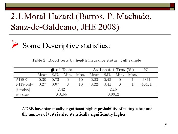
2. 1. Moral Hazard (Barros, P. Machado, Sanz-de-Galdeano, JHE 2008) Ø Some Descriptive statistics: ADSE have statistically significant higher probability of taking a test and the number of tests is also statistically significantly higher. 32

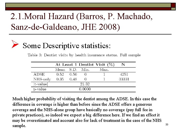
2. 1. Moral Hazard (Barros, P. Machado, Sanz-de-Galdeano, JHE 2008) Ø Some Descriptive statistics: Much higher probability of visiting the dentist among the ADSE. In this case the difference in coverage is higher than before since the ADSE offers a generous coverage and the NHS-alone group have basically no coverage (pay full fee in private practices), so indeed we expect a big difference here. If we find an effect it may be overestimated and account also for lack of treatment in the case of the NHS sample. 33

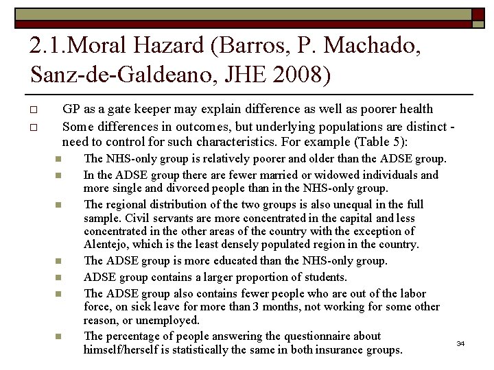
2. 1. Moral Hazard (Barros, P. Machado, Sanz-de-Galdeano, JHE 2008) GP as a gate keeper may explain difference as well as poorer health Some differences in outcomes, but underlying populations are distinct need to control for such characteristics. For example (Table 5): o o n n n n The NHS-only group is relatively poorer and older than the ADSE group. In the ADSE group there are fewer married or widowed individuals and more single and divorced people than in the NHS-only group. The regional distribution of the two groups is also unequal in the full sample. Civil servants are more concentrated in the capital and less concentrated in the other areas of the country with the exception of Alentejo, which is the least densely populated region in the country. The ADSE group is more educated than the NHS-only group. ADSE group contains a larger proportion of students. The ADSE group also contains fewer people who are out of the labor force, on sick leave for more than 3 months, not working for some other reason, or unemployed. The percentage of people answering the questionnaire about himself/herself is statistically the same in both insurance groups. 34

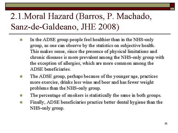
2. 1. Moral Hazard (Barros, P. Machado, Sanz-de-Galdeano, JHE 2008) n n In the ADSE group people feel healthier than in the NHS-only group, as one can observe by the statistics on subjective health. This makes sense, since the presence of physical limitations and chronic diseases is more prevalent among the NHS-only group with the exception of allergies, which are more common among the ADSE beneficiaries. The ADSE group, perhaps because of the younger age, practices more exercise, drinks less wine and beer and has fewer weight problems than the NHS-only group. The percentage of smokers is statistically the same in both groups. Finally, ADSE beneficiaries practice better dental hygiene than the NHS-only group. 35

2. 1. Moral Hazard (Barros, P. Machado, Sanz-de-Galdeano, JHE 2008) Why do we think the “treatment” (i. e ADSE coverage) is exogenous? Ø Unlikely that individuals anticipating high health care demand choose to become civil servants to obtain ADSE coverage, since they have coverage from the NHS. Ø People wish to become civil servants because they are employed for life and for some professions the State pays higher salaries. Ø Unlikely that the State chooses individuals on the basis of health. Individuals only have to go through a simple X-ray to discard tuberculosis (extremely rare nowadays as vaccine is compulsory and provided for free). Ø Other subsystems are more generous than ADSE (e. g. banking sector). Ø Finally, we think the unconfoundness assumption holds for the youngest generations although it may be violated for the eldest group => separate estimation by age groups. 36

2. 1. Moral Hazard (Barros, P. Machado, Sanz-de-Galdeano, JHE 2008) o o We estimate the Average Treatment Effect on the Treated (ATT) (Abadie and Imbens, 2006) i. e. Average increase in health care demand for ADSE beneficiaries due to their extra insurance. Matching estimators n n Avoid imposing functional form restrictions (allows for heterogeneous impact). Treatment group ADSE, control NHS-only 37

2. 1. Moral Hazard (Barros, P. Machado, Sanz-de-Galdeano, JHE 2008) Matching estimators: o Denote by Yi(0) the outcome of individual i, i=1, …N under the control group, and Yi(1) the outcome of the same individual under the treatment group. o Each individual is either in the control or the treatment group hence we only observe one of the Yi, i. e. either Yi(0) or Yi(1) depending of the treatment individual i has received. The unobserved outcome is the counterfactual that must be estimated. 38

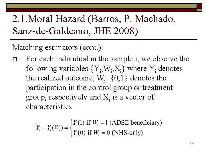
2. 1. Moral Hazard (Barros, P. Machado, Sanz-de-Galdeano, JHE 2008) Matching estimators (cont. ): o For each individual in the sample i, we observe the following variables {Yi, Wi, Xi} where Yi denotes the realized outcome, Wi={0, 1} denotes the participation in the control group or treatment group, respectively and Xi is a vector of characteristics. 39

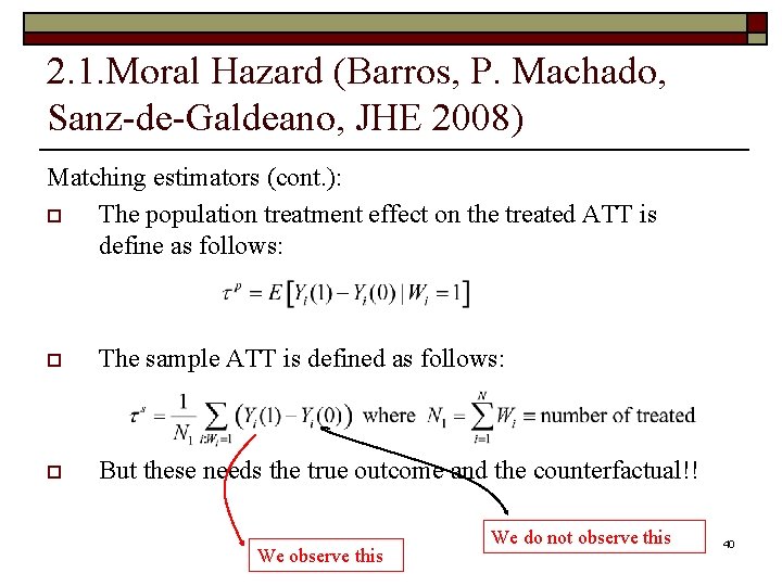
2. 1. Moral Hazard (Barros, P. Machado, Sanz-de-Galdeano, JHE 2008) Matching estimators (cont. ): o The population treatment effect on the treated ATT is define as follows: o The sample ATT is defined as follows: o But these needs the true outcome and the counterfactual!! We observe this We do not observe this 40

2. 1. Moral Hazard (Barros, P. Machado, Sanz-de-Galdeano, JHE 2008) Matching estimators (cont. ): o The main idea is that if assignment to treatment is independent of the potential outcome (conditional on the covariates), e. g. that individuals are not ADSE because they need more visits to the doctor, then we can use the outcome of similar individuals on the control group to input Yi(0). For these, we need that, conditional on the Xs, the ADSE beneficiaries be on average equal to the control group. n It cannot be, for example, that ADSE women of a certain age group and education that leave in Lisbon without any chronic disease are systematic more (or less) sick than another woman in the same conditions in the NHS-only group. In other words, the distribution of the unobservables e’s is similar for ADSE and NHS-only. Any difference in Y has to be due to treatment only. 41

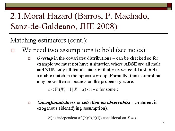
2. 1. Moral Hazard (Barros, P. Machado, Sanz-de-Galdeano, JHE 2008) Matching estimators (cont. ): o We need two assumptions to hold (see notes): o Overlap in the covariates distributions – can be checked so for example we must not have a situation where ADSE are all male and NHS-only all female since in that case we could not find a suitable match in the opposite group. Formally, this assumption may be written as bounds on the propensity score: o Unconfoundedness or selection on observables - treatment is exogenous (identifying assumption). 42

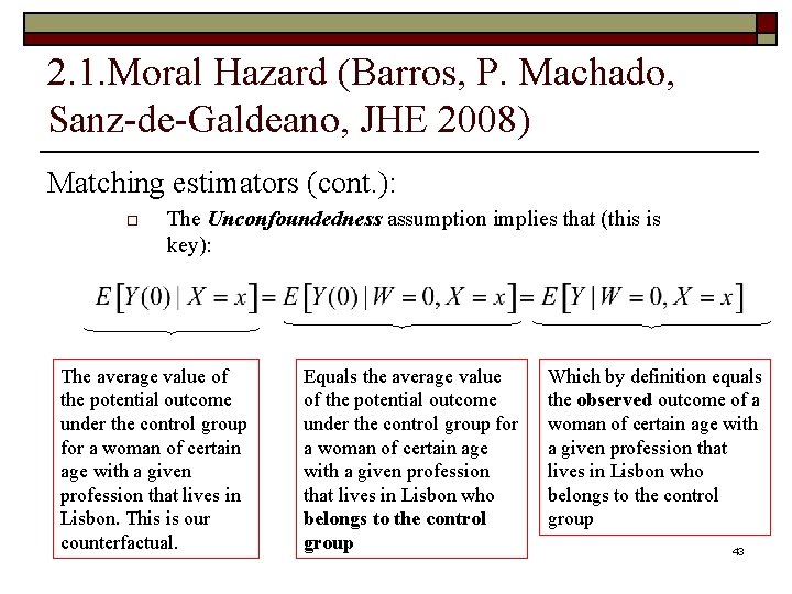
2. 1. Moral Hazard (Barros, P. Machado, Sanz-de-Galdeano, JHE 2008) Matching estimators (cont. ): o The Unconfoundedness assumption implies that (this is key): The average value of the potential outcome under the control group for a woman of certain age with a given profession that lives in Lisbon. This is our counterfactual. Equals the average value of the potential outcome under the control group for a woman of certain age with a given profession that lives in Lisbon who belongs to the control group Which by definition equals the observed outcome of a woman of certain age with a given profession that lives in Lisbon who belongs to the control group 43

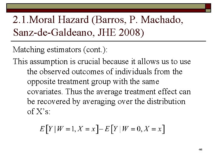
2. 1. Moral Hazard (Barros, P. Machado, Sanz-de-Galdeano, JHE 2008) Matching estimators (cont. ): This assumption is crucial because it allows us to use the observed outcomes of individuals from the opposite treatment group with the same covariates. Thus the average treatment effect can be recovered by averaging over the distribution of X’s: 44

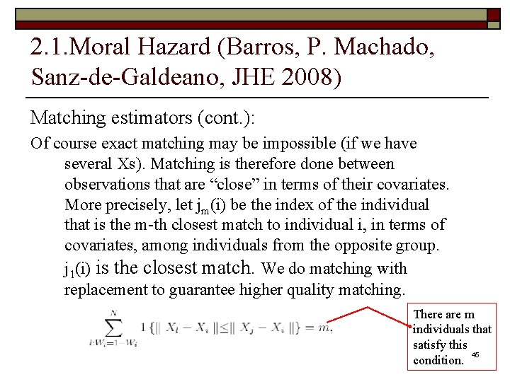
2. 1. Moral Hazard (Barros, P. Machado, Sanz-de-Galdeano, JHE 2008) Matching estimators (cont. ): Of course exact matching may be impossible (if we have several Xs). Matching is therefore done between observations that are “close” in terms of their covariates. More precisely, let jm(i) be the index of the individual that is the m-th closest match to individual i, in terms of covariates, among individuals from the opposite group. j 1(i) is the closest match. We do matching with replacement to guarantee higher quality matching. There are m individuals that satisfy this 45 condition.

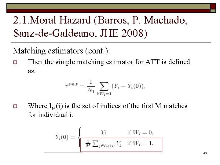
2. 1. Moral Hazard (Barros, P. Machado, Sanz-de-Galdeano, JHE 2008) Matching estimators (cont. ): o Then the simple matching estimator for ATT is defined as: o Where IM(i) is the set of indices of the first M matches for individual i: 46

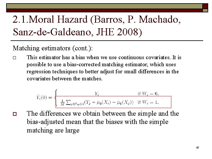
2. 1. Moral Hazard (Barros, P. Machado, Sanz-de-Galdeano, JHE 2008) Matching estimators (cont. ): o This estimator has a bias when we use continuous covariates. It is possible to use a bias-corrected matching estimator, which uses regression techniques to better adjust for small differences in the covariates between the matches. o The differences we obtain between the simple and the bias-adjusted mean that the biases with the simple matching are large 47

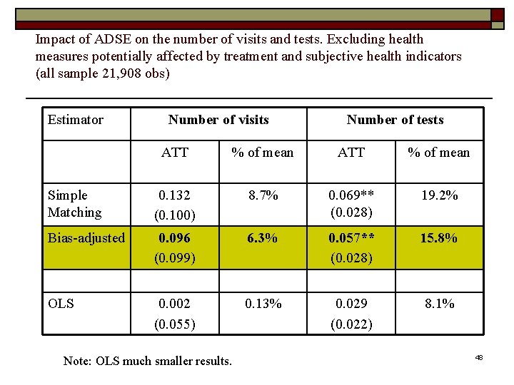
Impact of ADSE on the number of visits and tests. Excluding health measures potentially affected by treatment and subjective health indicators (all sample 21, 908 obs) Estimator Number of visits Number of tests ATT % of mean Simple Matching 0. 132 (0. 100) 8. 7% 0. 069** (0. 028) 19. 2% Bias-adjusted 0. 096 (0. 099) 6. 3% 0. 057** (0. 028) 15. 8% OLS 0. 002 (0. 055) 0. 13% 0. 029 (0. 022) 8. 1% Note: OLS much smaller results. 48

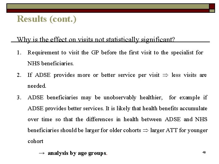
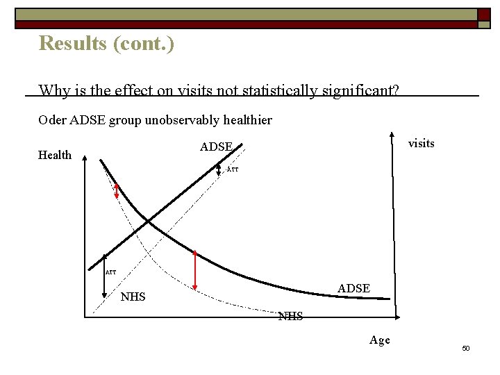
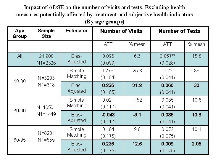
Results (cont. ) Why is the effect on visits not statistically significant? 1. Requirement to visit the GP before the first visit to the specialist for NHS beneficiaries. 2. If ADSE provides more or better service per visit less visits are needed. 3. ADSE beneficiaries may be unobservably healthier, for example if ADSE provides better services. It is likely that health benefits accumulate over time so that the differences in health between ADSE and NHS beneficiaries should be larger for older cohorts larger ATT for younger cohort → analysis by age groups. 49

Results (cont. ) Why is the effect on visits not statistically significant? Oder ADSE group unobservably healthier visits ADSE Health ATT ADSE NHS Age 50

Impact of ADSE on the number of visits and tests. Excluding health measures potentially affected by treatment and subjective health indicators (By age groups) Age Group All 18 -30 30 -60 60 -95 Sample Size 21, 908 N 1=2326 N=3203 N 1=318 N=10501 N 1=1449 N=8204 N 1=559 Estimator Number of Visits Number of Tests ATT % mean Bias. Adjusted 0. 096 (0. 099) 6. 3 0. 057** (0. 028) 15. 8 Simple Matching 0. 279* (0. 164) 25. 8 0. 072* (0. 041) 36 Bias. Adjusted 0. 235 (0. 165) 21. 8 0. 060 (0. 041) 30 Simple Matching 0. 021 (0. 117) 1. 52 0. 035 (0. 041) 10. 6 Bias. Adjusted -0. 043 (0. 117) -3. 1 0. 036 (0. 041) 10. 9 Simple Matching 0. 184 (0. 175) 9. 8 0. 072 (0. 075) 16. 4 Bias. Adjusted 0. 236 (0. 175) 12. 6 0. 009 (0. 075) 2. 05 51

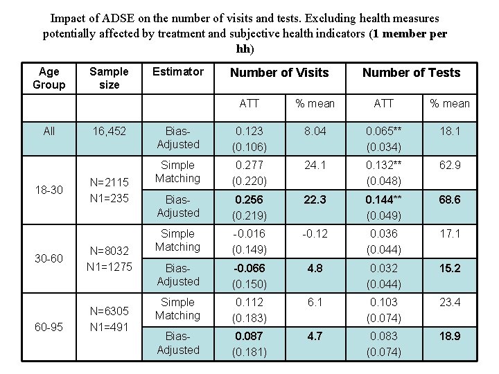
Impact of ADSE on the number of visits and tests. Excluding health measures potentially affected by treatment and subjective health indicators (1 member per hh) Age Group All 18 -30 30 -60 60 -95 Sample size 16, 452 N=2115 N 1=235 N=8032 N 1=1275 N=6305 N 1=491 Estimator Number of Visits Number of Tests ATT % mean Bias. Adjusted 0. 123 (0. 106) 8. 04 0. 065** (0. 034) 18. 1 Simple Matching 0. 277 (0. 220) 24. 1 0. 132** (0. 048) 62. 9 Bias. Adjusted 0. 256 (0. 219) 22. 3 0. 144** (0. 049) 68. 6 Simple Matching -0. 016 (0. 149) -0. 12 0. 036 (0. 044) 17. 1 Bias. Adjusted -0. 066 (0. 150) 4. 8 0. 032 (0. 044) 15. 2 Simple Matching 0. 112 (0. 183) 6. 1 0. 103 (0. 074) 23. 4 Bias. Adjusted 0. 087 (0. 181) 4. 7 0. 083 (0. 074) 18. 9 52

Robustness Checks on the exogeneity of ADSE Ø Note: need to show quality of the matching (table 10 in the paper) Ø Are ADSE beneficiaries more risk averse? Ø Run ols regressions of risky health habits Ø (smoking/drinking) against X’s and ADSE dummy. ADSE beneficiaries consumed more wine but less whisky. No differences in smoking behavior. Run probit on prevention and brushing teeth – no effect Ø Do individuals with ADSE under their name behave differently than family members? 53

On the exogeneity of the insurance plan ØIdea: If there is adverse selection the impact of ADSE should not be similar for those holding it in their own name (moral hazard + adverse selection) those that have it in the name of a family member (only moral hazard). Ø Unfortunately the dataset does not have information on whether an individual has ADSE in his own name or through family. So use subsample of unemployed (who by definition must have ADSE through a family member) and compare with unemployed NHS beneficiaries. 54

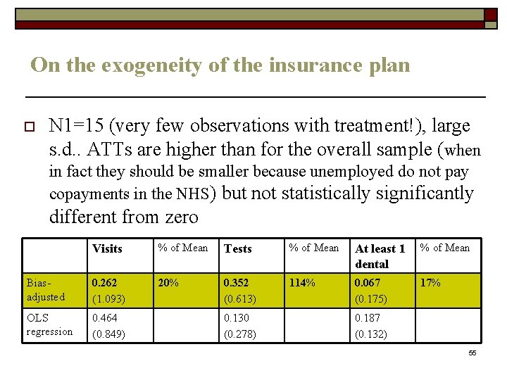
On the exogeneity of the insurance plan o N 1=15 (very few observations with treatment!), large s. d. . ATTs are higher than for the overall sample (when in fact they should be smaller because unemployed do not pay copayments in the NHS) but not statistically significantly different from zero Visits % of Mean Tests % of Mean At least 1 dental % of Mean Biasadjusted 0. 262 (1. 093) 20% 0. 352 (0. 613) 114% 0. 067 (0. 175) 17% OLS regression 0. 464 (0. 849) 0. 130 (0. 278) 0. 187 (0. 132) 55

Conclusion 1. Effects of additional coverage are positive and large. 2. ATT estimates for the whole sample: 0. 096 (6%) for visits, 0. 057** (15. 8%) for tests, and 0. 019 (7%) for dentist. 3. Effects are larger for the youngest age group: 21. 8 -22. 3% for visits, 30 -68%** for tests, and 11. 6% for dentists. 4. Effects are smaller and not statistically significantly different from zero for other age-groups. 5. Moral hazard for “tests” but not clear for “visits”. No moral hazard for dentist visits. 56