The importance of mixed selectivity in complex cognitive

The importance of mixed selectivity in complex cognitive tasks Mattia Rigotti - Omri Barak - Melissa R. Warden - Xiao-Jing Wang - Nathaniel D. Daw - Earl K. Miller - Stefano Fusi Presented by Nicco Reggente for BNS Cognitive Journal Club – 2/18/14

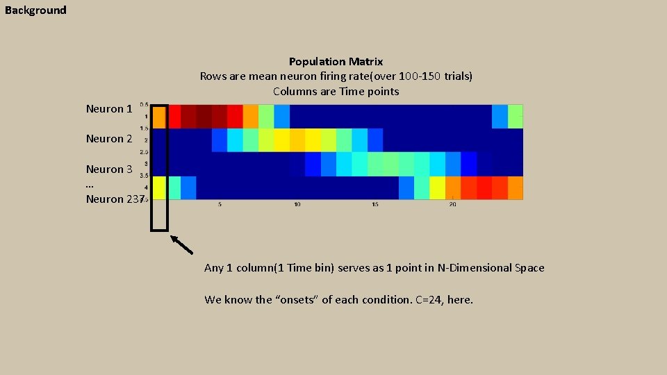
Background Population Matrix Rows are mean neuron firing rate(over 100 -150 trials) Columns are Time points Neuron 1 Neuron 2 Neuron 3 … Neuron 237 Any 1 column(1 Time bin) serves as 1 point in N-Dimensional Space We know the “onsets” of each condition. C=24, here.

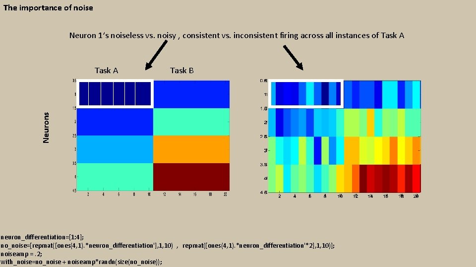
The importance of noise Neuron 1’s noiseless vs. noisy , consistent vs. inconsistent firing across all instances of Task A Task B Neurons Task A neuron_differentiation=[1: 4]; no_noise=[repmat([ones(4, 1). *neuron_differentiation'], 1, 10) , repmat([ones(4, 1). *neuron_differentiation'*2], 1, 10)]; noiseamp =. 2; with_noise=no_noise + noiseamp*randn(size(no_noise));

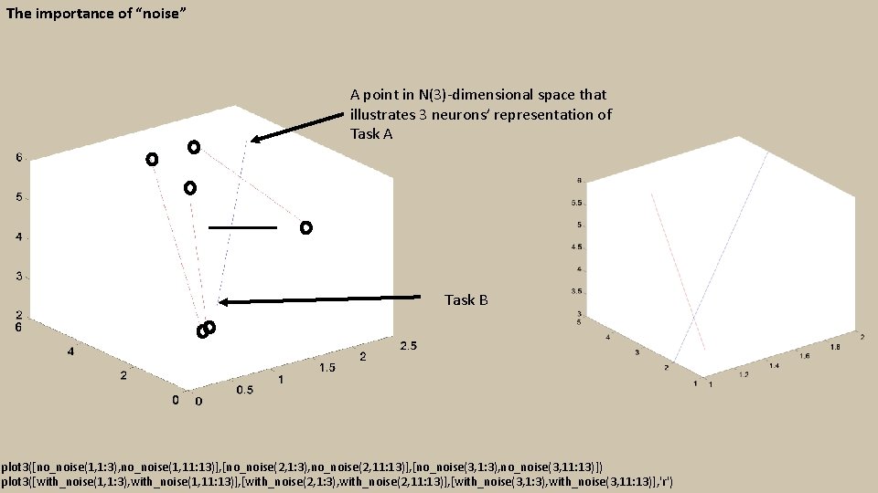
The importance of “noise” A point in N(3)-dimensional space that illustrates 3 neurons’ representation of Task A Task B plot 3([no_noise(1, 1: 3), no_noise(1, 11: 13)], [no_noise(2, 1: 3), no_noise(2, 11: 13)], [no_noise(3, 1: 3), no_noise(3, 11: 13)]) plot 3([with_noise(1, 1: 3), with_noise(1, 11: 13)], [with_noise(2, 1: 3), with_noise(2, 11: 13)], [with_noise(3, 1: 3), with_noise(3, 11: 13)], 'r')

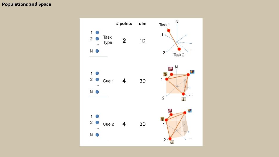
Populations and Space

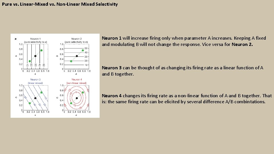
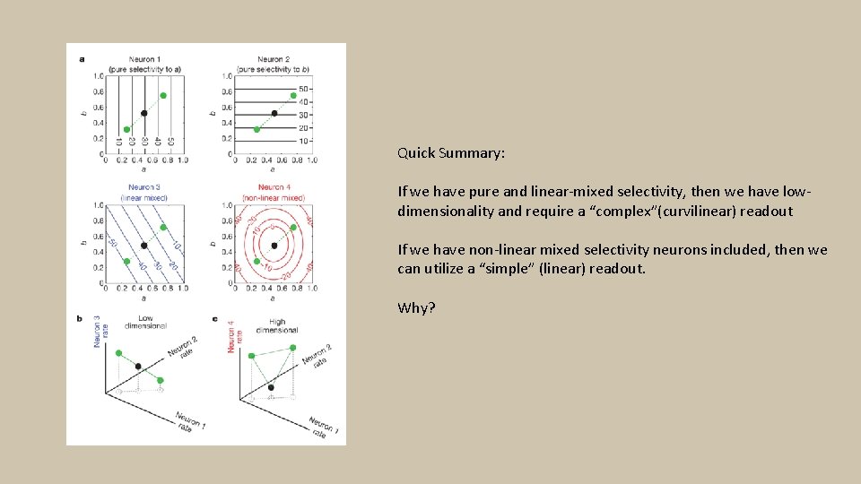
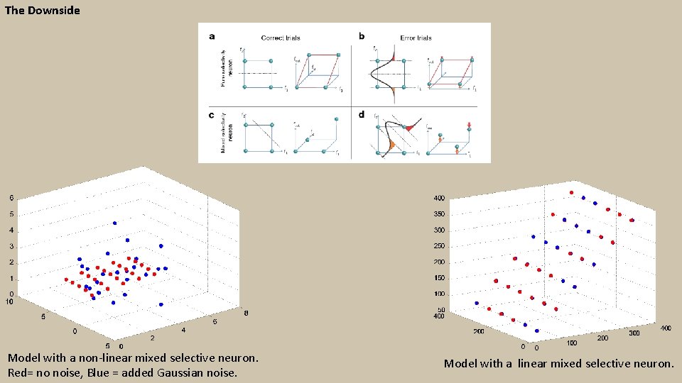
Pure vs. Linear-Mixed vs. Non-Linear Mixed Selectivity Neuron 1 will increase firing only when parameter A increases. Keeping A fixed and modulating B will not change the response. Vice versa for Neuron 2. Neuron 3 can be thought of as changing its firing rate as a linear function of A and B together. Neuron 4 changes its firing rate as a non-linear function of A and B together. That is: the same firing rate can be elicited by several difference A/B combintations.

A Population of “pure selectivity” neurons Low Dimensionality x=[]; y=[]; z=[]; for a=1: 5 for b=1: 5 neuron_1_function=60*a + 0*b; neuron_2_function=60*b+0*a; neuron_3_function=60+3*b; x=[x neuron_1_function]; y=[y neuron_2_function]; z=[z neuron_3_function]; end scatter 3(x, y, z, 'r', 'fill') We only need a two-coordinate axis to specify the position of these points. The points do not span all 3 dimensions.

A Population of “pure and linear mixed selectivity” neurons Low Dimensionality x=[]; y=[]; z=[]; for a=1: 5 for b=1: 5 neuron_1_function=60*a + 0*b; neuron_2_function=60*b+0*a; neuron_3_function=60*a+3*b; x=[x neuron_1_function]; y=[y neuron_2_function]; z=[z neuron_3_function]; end scatter 3(x, y, z, 'r', 'fill') Still…. We only need a twocoordinate axis to specify the position of these points. The points do not span all 3 dimensions.

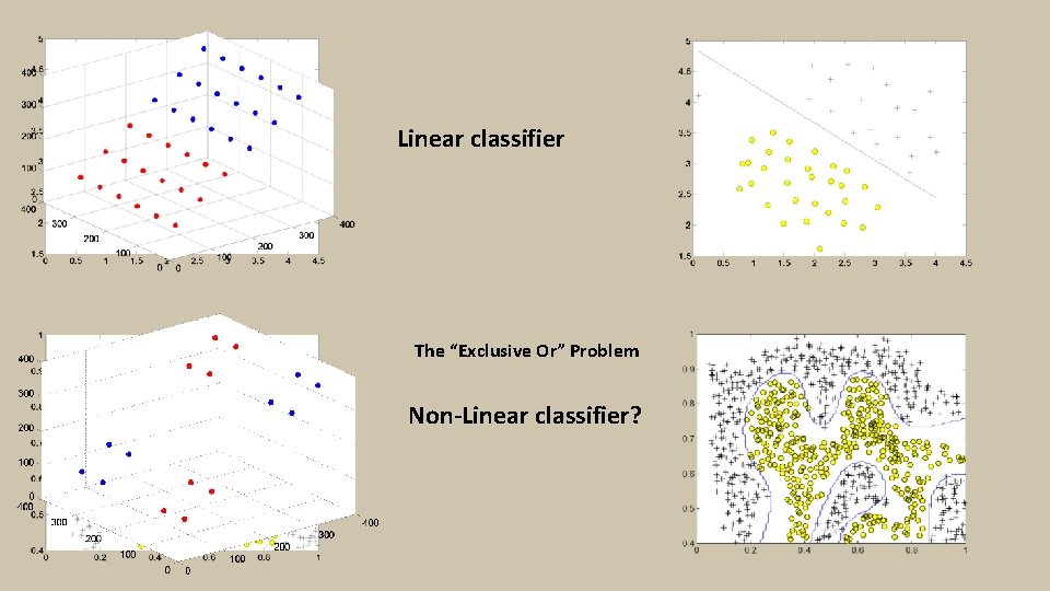
Linear classifier The “Exclusive Or” Problem Non-Linear classifier?

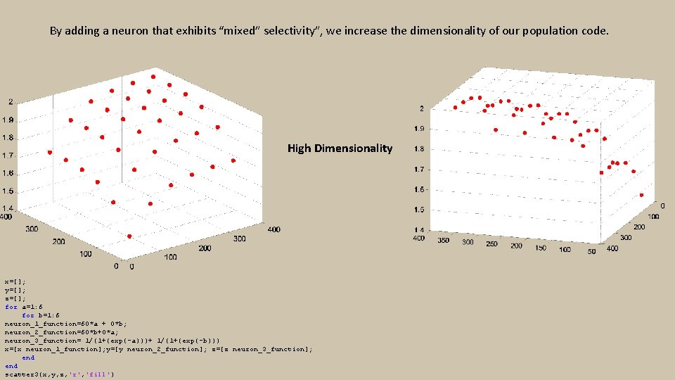
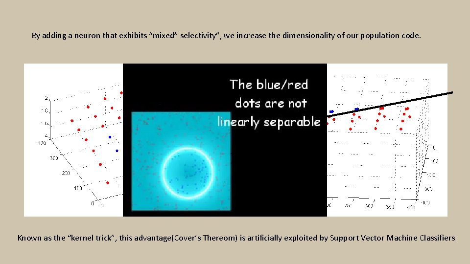
By adding a neuron that exhibits “mixed” selectivity”, we increase the dimensionality of our population code. High Dimensionality x=[]; y=[]; z=[]; for a=1: 6 for b=1: 6 neuron_1_function=60*a + 0*b; neuron_2_function=60*b+0*a; neuron_3_function= 1/(1+(exp(-a)))+ 1/(1+(exp(-b))) x=[x neuron_1_function]; y=[y neuron_2_function]; z=[z neuron_3_function]; end scatter 3(x, y, z, 'r', 'fill')

By adding a neuron that exhibits “mixed” selectivity”, we increase the dimensionality of our population code. Known as the “kernel trick”, this advantage(Cover’s Thereom) is artificially exploited by Support Vector Machine Classifiers

Quick Summary: If we have pure and linear-mixed selectivity, then we have lowdimensionality and require a “complex”(curvilinear) readout If we have non-linear mixed selectivity neurons included, then we can utilize a “simple” (linear) readout. Why?

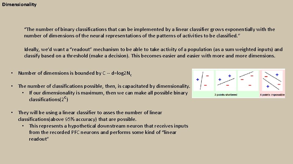
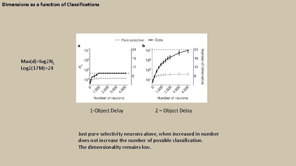
Dimensionality “The number of binary classifications that can be implemented by a linear classifier grows exponentially with the number of dimensions of the neural representations of the patterns of activities to be classified. ” Ideally, we’d want a “readout” mechanism to be able to take activity of a population (as a sum weighted inputs) and classify based on a threshold (make a decision). This becomes easier and easier with more and more dimensions. • Number of dimensions is bounded by C -- d=log 2 Nc • The number of classifications possible, then, is capacitated by dimensionality. • If our dimensionality is maximum, then we can make all possible binary classifications(2 c) • They will be using a linear classifier to asses the number of linear classifications(above 95% accuracy) that are possible. • This represents a hypothetical downstream neuron that receives inputs from the recorded PFC neurons and performs some kind of “linear readout”

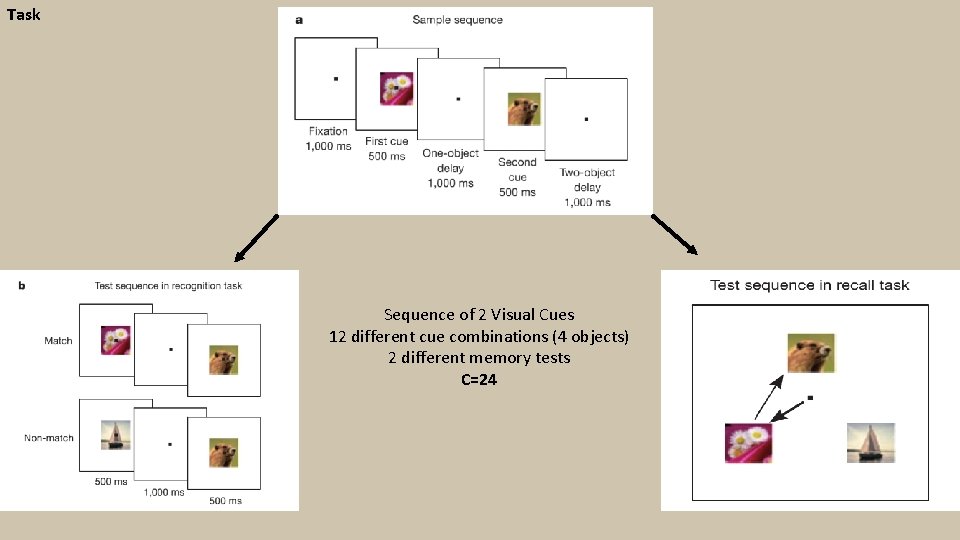
Task Sequence of 2 Visual Cues 12 different cue combinations (4 objects) 2 different memory tests C=24

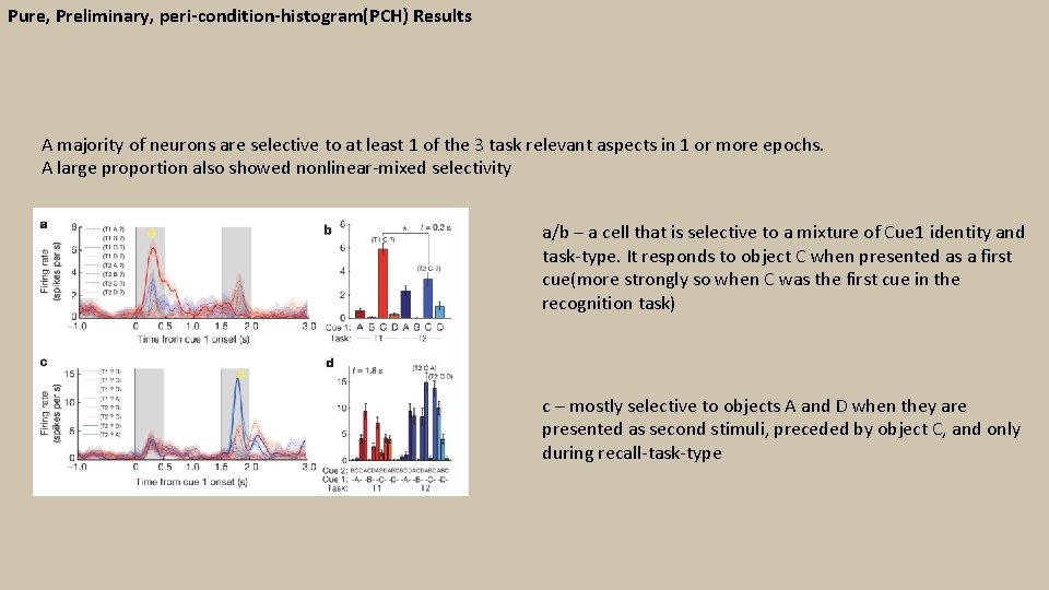
Pure, Preliminary, peri-condition-histogram(PCH) Results A majority of neurons are selective to at least 1 of the 3 task relevant aspects in 1 or more epochs. A large proportion also showed nonlinear-mixed selectivity a/b – a cell that is selective to a mixture of Cue 1 identity and task-type. It responds to object C when presented as a first cue(more strongly so when C was the first cue in the recognition task) c – mostly selective to objects A and D when they are presented as second stimuli, preceded by object C, and only during recall-task-type

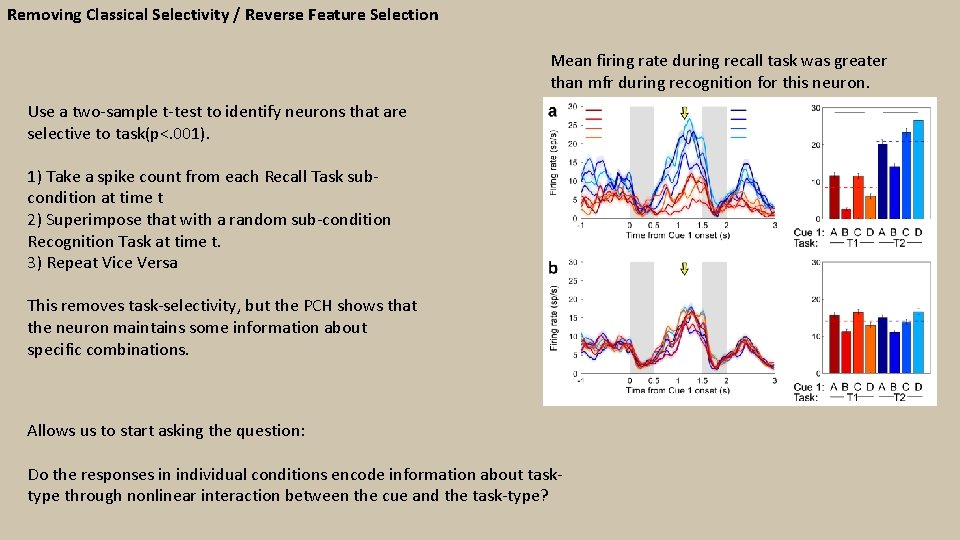
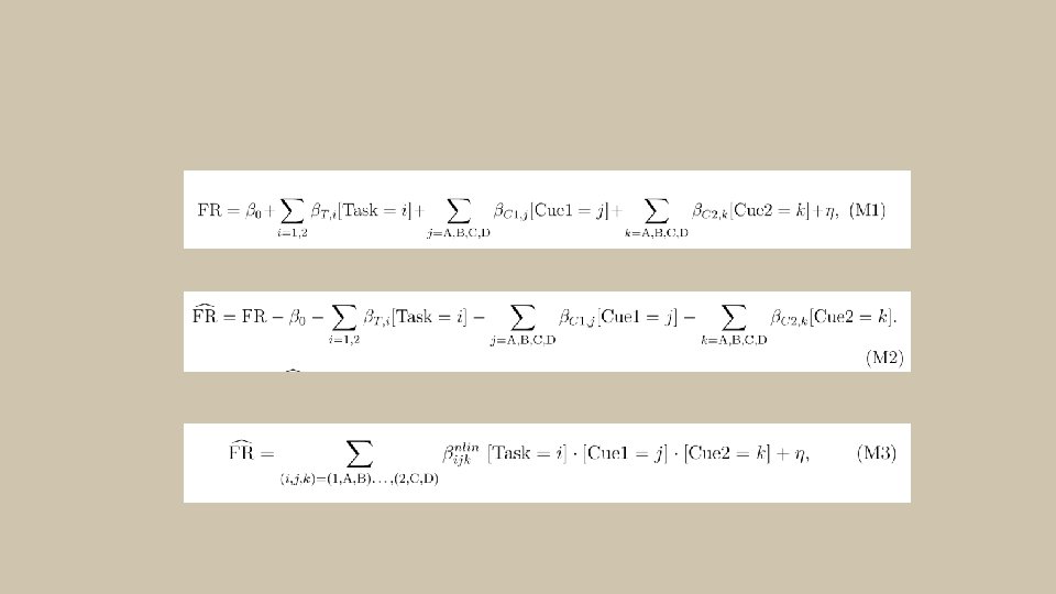
Removing Classical Selectivity / Reverse Feature Selection Mean firing rate during recall task was greater than mfr during recognition for this neuron. Use a two-sample t-test to identify neurons that are selective to task(p<. 001). 1) Take a spike count from each Recall Task subcondition at time t 2) Superimpose that with a random sub-condition Recognition Task at time t. 3) Repeat Vice Versa This removes task-selectivity, but the PCH shows that the neuron maintains some information about specific combinations. Allows us to start asking the question: Do the responses in individual conditions encode information about tasktype through nonlinear interaction between the cue and the task-type?

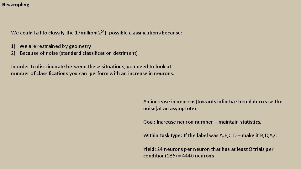
Resampling We could fail to classify the 17 million(224) possible classifications because: 1) We are restrained by geometry 2) Because of noise (standard classification detriment) In order to discriminate between these situations, you need to look at number of classifications you can perform with an increase in neurons. An increase in neurons(towards infinity) should decrease the noise(at an asymptote). Goal: Increase neuron number + maintain statistics. Within task type: If the label was A, B, C, D – make it B, D, A, C Yield: 24 neurons per neuron that has at least 8 trials per condition(185) = 4440 neurons

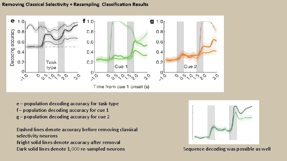
Removing Classical Selectivity + Resampling Classification Results e – population decoding accuracy for task-type f – population decoding accuracy for cue 1 g – population decoding accuracy for cue 2 Dashed lines denote accuracy before removing classical selectivity neurons Bright solid lines denote accuracy after removal Dark solid lines denote 1, 000 re-sampled neurons Sequence decoding was possible as well

Dimensions as a function of Classifications Max(d)=log 2 Nc Log 2(17 M)=24 Just pure selectivity neurons alone, when increased in number does not increase the number of possible classification. The dimensionality remains low.

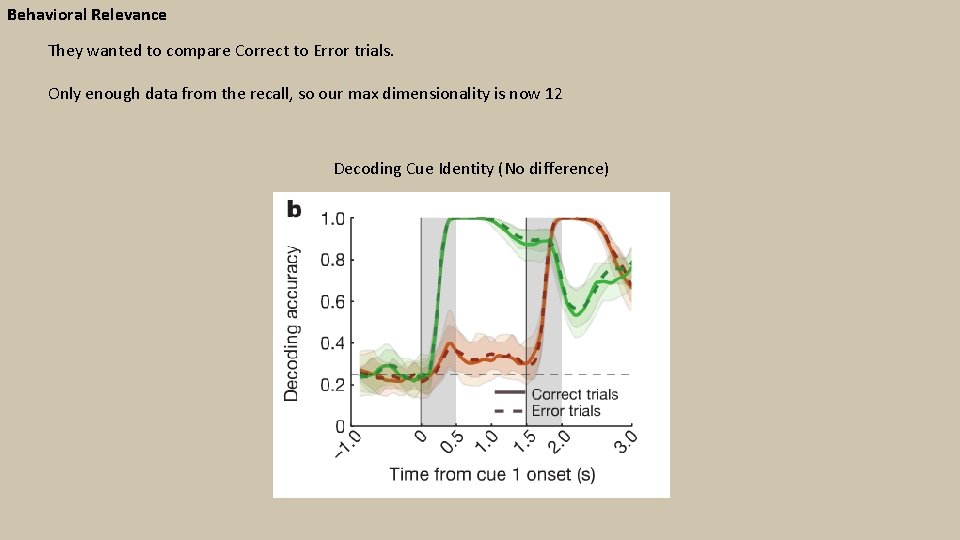
Behavioral Relevance They wanted to compare Correct to Error trials. Only enough data from the recall, so our max dimensionality is now 12 Decoding Cue Identity (No difference)

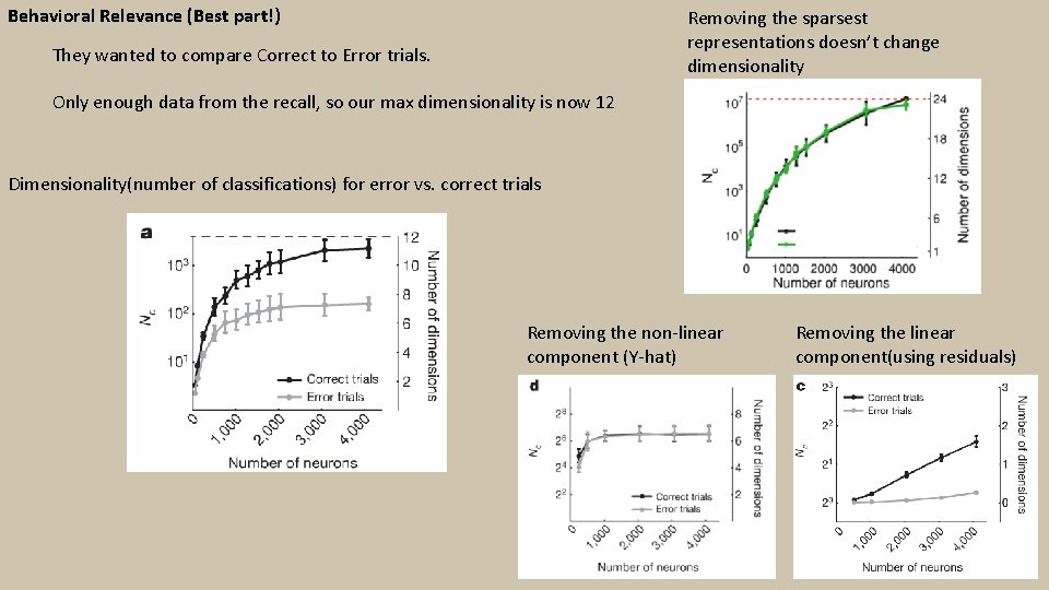
Behavioral Relevance (Best part!) Removing the sparsest representations doesn’t change dimensionality They wanted to compare Correct to Error trials. Only enough data from the recall, so our max dimensionality is now 12 Dimensionality(number of classifications) for error vs. correct trials Removing the non-linear component (Y-hat) Removing the linear component(using residuals)

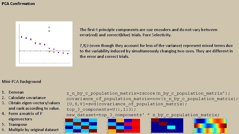
PCA Confirmation The first 6 principle components are cue encoders and do not vary between error(red) and correct(blue) trials. Pure Selectivity. 7, 8, 9 (even though they account for less of the variance) represent mixed terms due to the variability induced by simultaneously changing two cues. They are different in the error and correct trials. Mini-PCA Background 1. Demean 2. Calculate covariance 3. Obtain eigen-vectors/values and rank according to value. 4. Form a matrix of P eigenvectors 5. Transpose 6. Multiple by original dataset z_n_by_c_population_matrix=zscore(n_by_c_population_matrix'); covariance_of_population_matrix=cov(z_n_by_c_population_matrix); [U, S, V]=svd(covariance_of_population_matrix); top_3_components=U(: , 1: 3); new_dataset=top_3_components' * n_by_c_population_matrix;

The Downside Model with a non-linear mixed selective neuron. Red= no noise, Blue = added Gaussian noise. Model with a linear mixed selective neuron.

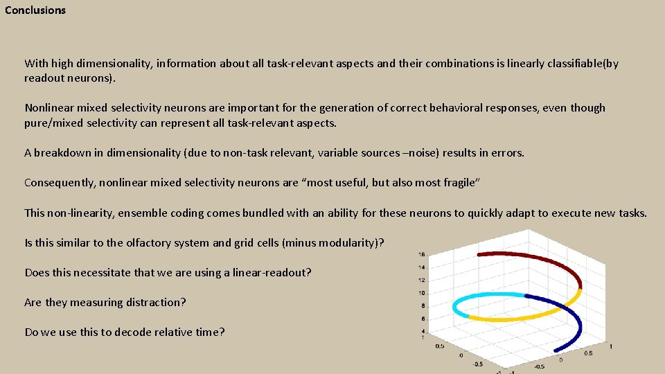
Conclusions With high dimensionality, information about all task-relevant aspects and their combinations is linearly classifiable(by readout neurons). Nonlinear mixed selectivity neurons are important for the generation of correct behavioral responses, even though pure/mixed selectivity can represent all task-relevant aspects. A breakdown in dimensionality (due to non-task relevant, variable sources –noise) results in errors. Consequently, nonlinear mixed selectivity neurons are “most useful, but also most fragile” This non-linearity, ensemble coding comes bundled with an ability for these neurons to quickly adapt to execute new tasks. Is this similar to the olfactory system and grid cells (minus modularity)? Does this necessitate that we are using a linear-readout? Are they measuring distraction? Do we use this to decode relative time?

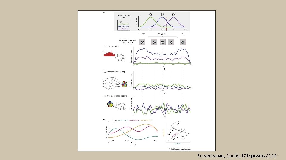
Sreenivasan, Curtis, D’Esposito 2014

More on PCA A matrix multipled by a vector is treating the matrix as a transformation matrix that changes the vector in some way. The nature of a transformation gives rise to eigenvectors o If you take a matrix, apply to it some vector and the resulting vector lays on the same line as the applied vector, then it is a reflected vector. o A vector that causes the transformation matrix to have this reflected vector would be considered an eigenvector of that transformation matrix (so would all multiples of it. ) Eigenvectors can only be found for square matrices. o Not every square matrix has eigenvectors o For an nxn matrix that has eigenvectors, there are n of them. E. g if a mtrix is 3 x 3 and has eigenvectors…it has 3 of them. o All eigenvectors of a matrix are perpendicular to each other no matter how many dimensions you have. Orthogonality. o Mathemiticians prefer to find eigenvectors whose length is exactly one. The length of a vector doesn’t affect it, but direction does. So, we want to scale it to have a length of 1. o We can find the length of an eigenvector by taking the square root of the summed squares of all the numbers in the vector. If we divide the original sector by the above value, we can make it have a length of 1. o SVD will return the eigenvectors in its U. Each column will be an eigenvector of the supplied matrix. Eigenvalues o The value that can be multiplied to the eigenvector that will yield the resulting vector after a matrix has been multiplied by its eigenvector. E. g if A is a matrix and v is its eigenvector and B is the resulting vector of their multiplication, then the eigenvalue times v will result in B as well. o SVD will give us the eigenvalues in the S column.

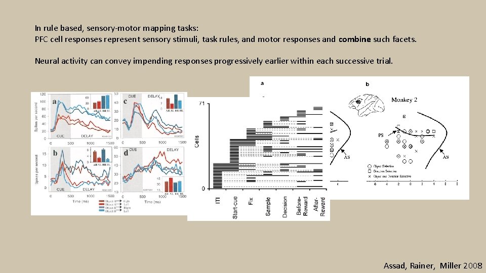
In rule based, sensory-motor mapping tasks: PFC cell responses represent sensory stimuli, task rules, and motor responses and combine such facets. Neural activity can convey impending responses progressively earlier within each successive trial. Assad, Rainer, Miller 2008