The Fundamentals of Political Science Research 2 nd

The Fundamentals of Political Science Research, 2 nd Edition Chapter 6: Probability and Statistical Inference

Chapter 6 Outline • 1 Populations and samples • 2 Some Basics of Probability Theory • 3 Learning about the population from a sample: The central limit theorem • 4 Example: Presidential approval ratings • 5 What kind of sample was that? • 6 A note on the effect of sample size • 7 A Look Ahead: Examining Relationships Between Variables

Looking back, looking ahead • We now know how to use descriptive statistics --that is, measures of central tendency and measures of dispersion—to “describe" what a distribution of data looks like. • For example, we can describe a class's scores on an exam or a paper with things like the mode, median and mean, and its standard deviation.

Populations versus samples • But we also know that many of our statistics are derived from samples of data. We've said that we tend not to care about our samples in and of themselves, but only insofar as they tell us something about the population as a whole.

This is statistical inference • Statistical inference is the process of making probabilistic statements about a population characteristic based on our knowledge of the sample characteristic. • In other words, there are things we know about with certainty—like the mean of some variable in our sample. But we care about the likely values of that variable in the entire population. Since we almost never have data for an entire population, we need to use what we know to infer the likely range of values in the population.

How is that possible? • If we only see a sample of data--even a randomly selected sample--how can we possibly know anything about the vast majority of individuals for whom we don't have data? • There is a way, and its called the Central Limit Theorem. • First, though, a detour into some probability theory.

An example • Suppose that you have a pillowcase with 550 blue beads and 450 red beads in it. • You have a friend reach her hand into the pillowcase—no peeking!--and have her draw out 100 beads, and then count the red and blue beads. • She happened to draw 46 red beads and 54 blue ones. • The key question: Based on her count, what is her best guess about the percentage of red beads versus blue beads in the entire pillowcase?

How the laws of probability apply • In the above example, the laws of probability are useful for taking particular information about a characteristic of an observed sample of data and attempting to generalize that information to the underlying and unobserved population. • The observed sample above, of course, is the sample of 100 that your friend drew from the pillowcase. • The underlying population is represented by the 1000 beads in the bag.

Definitions • An outcome is the result of a random observation. • Two or more outcomes can be said to be independent outcomes if the realization of one of the outcomes does not affect the realization of the other outcomes. (For example, the roll of two dice represents independent outcomes, because the outcome of the first die does not affect the outcome of the second die. )

Properties of probability • 1 All outcomes have some probability ranging from 0 to 1. • 2 The sum of all possible outcomes must be exactly 1. • 3 If (but only if!) two outcomes are independent, then the probability of those events both occurring is equal to the product of them individually. So, if we have a fair coin, and toss it three times—and be mindful that each toss is an independent outcome--the probability of tossing three tails is 1/2 X 1/2 = 1/8.

Remember the goal • There are some things (like the mean) that we can know (with certainty) about a sample. But we care about the population. How can we learn about the population from a sample? • That process is called “statistical inference. " • The Central Limit Theorem will invoke a particular kind of distribution called the normal distribution, with which most of you are casually familiar. It's also called a bell-shaped distribution. But it has some unique features.

The normal distribution • The Central Limit Theorem will invoke a particular kind of distribution called the normal distribution, with which most of you are casually familiar. It's also called a bellshaped distribution. But it has some unique features.

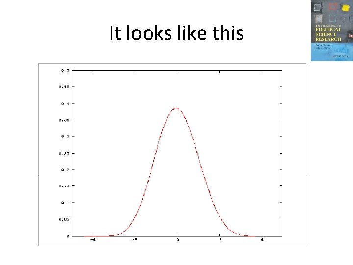
What is a “normal” distribution? • “Normal" does not mean “typical, " or “good, " or whatever. Its opposite is not the “abnormal" distribution or the “deviant“ distribution. (Technically, distributions do not have opposites. ) • It is a distribution that is symmetrical, so that the mode, median, and mean are all equal. (But not all symmetrical distributions are normal. ) It also has certain properties that are useful.

It looks like this

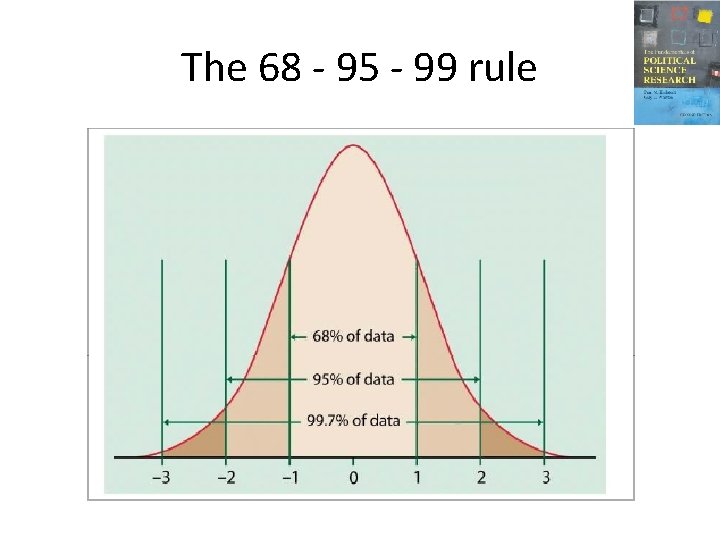
Why is it useful? • Because, if a distribution is normally shaped, we know a certain % of cases fall within a certain distance of the mean.

The 68 - 95 - 99 rule

Are all distributions normal? • NO! • A frequency distribution is just a distribution of scores (like your scores on the midterm, or the distribution of income in Nebraska). • Most frequency distributions are not normally shaped.

But… • Even if a frequency distribution is not normally shaped, if we imagine a (hypothetical) world in which we took an infinite number of samples, and took the mean of each sample, and then plotted those means, then how would those plotted means be distributed?

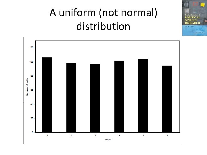
An example • Imagine that we rolled a six-sided dice like you play a game of Clue with. It can come out as a 1, 2, 3, 4, 5 or 6 with equal probability, right? • Let's say you rolled that dice 600 times. What would that distribution “look like"?

A uniform (not normal) distribution

That’s not normal • That's not normal, right? • Let's say we rolled that dice 600 times. What do you think the mean would be (about)? • Would it be exactly 3. 5? Every time? No, of course not. • But what would happen if we did that roll-it 600 -times thing, say, a billion times, then plotted the means? (Not the rolls, the means. Be careful!)

It would be normal • Think about this carefully. In our frequency distribution, we could get a score of 1 to 6 with equal likelihood. But in our sample means, we would never get means of 1 or 6. All of our means would be somewhere around 3. 5, yes? Moreover, they would be distributed around that mean (3. 5) normally.

This is the Central Limit Theorem • The Central Limit Theorem says that, no matter what the underlying shape of the frequency distribution (whether it's uniform, normal, or whatever), the hypothetical distribution of sample means--which is called a sampling distribution--will be normal, with mean equal to the true population mean, and standard deviation equal to The above is called the standard error of the mean.

Then… • You can use what you know about the sample to infer what is likely to be true about the population.

A polling result from October 2006 • On October 5 and 6, 2006, Newsweek magazine sponsored a survey in which 1, 004 randomly selected Americans were interviewed about their political beliefs. Among the questions they asked was the following item intended to tap into a respondent's evaluation of the president's job performance: – “Do you approve or disapprove of the way George W. Bush is handling his job as president? "

The results • In early October, 2006, 33% of the sample approved of Bush's job performance, 59% disapproved, and 8% were unsure. • We're only interested in the opinions of those 1, 004 Americans who happened to be in the sample insofar as they tell us something about the adult population as a whole. But we can use these 1, 004 responses to do precisely that, using the logic of the central limit theorem.

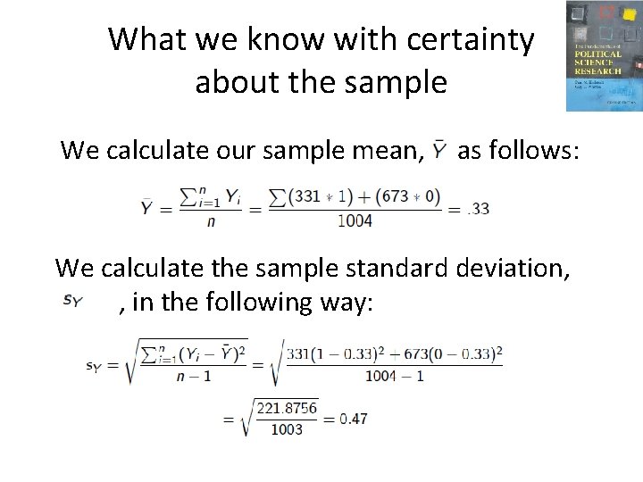
What we know with certainty about the sample We calculate our sample mean, as follows: We calculate the sample standard deviation, , in the following way:

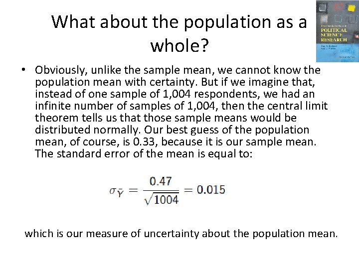
What about the population as a whole? • Obviously, unlike the sample mean, we cannot know the population mean with certainty. But if we imagine that, instead of one sample of 1, 004 respondents, we had an infinite number of samples of 1, 004, then the central limit theorem tells us that those sample means would be distributed normally. Our best guess of the population mean, of course, is 0. 33, because it is our sample mean. The standard error of the mean is equal to: which is our measure of uncertainty about the population mean.

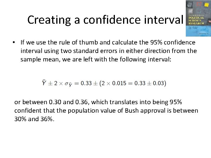
Creating a confidence interval • If we use the rule of thumb and calculate the 95% confidence interval using two standard errors in either direction from the sample mean, we are left with the following interval: or between 0. 30 and 0. 36, which translates into being 95% confident that the population value of Bush approval is between 30% and 36%.

Those plus-or-minus figures • This is where the “plus-or-minus" figures that we always see in public opinion polls come from. • The best guess for the population mean value is the sample mean value, plus or minus two standard errors. • So the plus-or-minus figures we are accustomed to seeing are built, typically, on the 95% interval.

Random samples vs. samples of convenience • The central limit theorem only applies to samples that are selected randomly. With a sample of convenience, by contrast, we cannot invoke the central limit theorem to construct a sampling distribution and create a confidence interval. • A non-randomly selected sample of convenience does very little to help us build bridges between the sample and the population about which we want to learn. What do such “surveys" say about the population as a whole? Because their samples are clearly not random samples of the underlying population, the answer is “nothing. "

How much does sample size matter? • As the formula for the confidence interval indicates, the smaller the standard errors, the “tighter" our resulting confidence intervals will be, and larger standard errors will produce “wider" confidence intervals. • If we are interested in estimating population values, based on our samples, with as much precision as possible, then it is desirable to have tighter instead of wider confidence intervals.

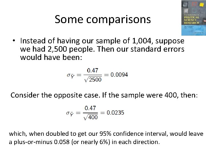
Some comparisons • Instead of having our sample of 1, 004, suppose we had 2, 500 people. Then our standard errors would have been: Consider the opposite case. If the sample were 400, then: which, when doubled to get our 95% confidence interval, would leave a plus-or-minus 0. 058 (or nearly 6%) in each direction.

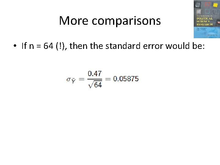
More comparisons • If n = 64 (!), then the standard error would be:

A look ahead • In this chapter, all we have done is talk about the process of statistical inference with a single variable. • In Chapter 7, you will learn three different ways to move into the world of bivariate hypothesis testing. We will examine relationships between two variables, typically in a sample, and then make probabilistic assessments of the likelihood that those relationships exist in the population. • The logic is identical to what you have just learned; we merely extend it to cover relationships between two variables. • After that, in Chapter 8, you will learn one other way to conduct hypothesis tests involving two variables--the bivariate regression model.