Technological Change and Economic Growth the Interwar Years

Technological Change and Economic Growth: the Interwar Years and the 1990 s Alexander J. Field afield@scu. edu All Ohio Eocnomic History Seminar Ohio State Universiyty April 30, 2004

The Most Technologically Progressive Decade of the Century n n Field, American Economic Review (2003) Hint #1: It’s not what you think … Hint #2: It wasn’t the 1990 s. . . Hint #3: It wasn’t the 1920 s…

The Main Argument n The years 1929 -1941 were, in the aggregate, the most technologically progressive of any comparable period in U. S. economic history.

Labor and Multifactor Productivity Growth Formulas Y = real output N= labor hours K=capital input Y/N = Labor Productivity y – n = Labor Productivity growth (lower case letters = compound annual average rates of growth) Y = A KβN 1 -β = Production function (Cobb Douglas, crts) A = Y/(KβN 1 -β) = Multifactor Productivity a = y – βk – (1 -β)n = Growth Rate of MFP y - n = a + β (k - n) = Growth rate of labor productivity

Disclaimers - 1 n What we measure in the residual contains not only serendipitous or accidental discovery of useful knowledge, but a variety of related influences, including, but not limited to: • The outcomes of focused research and development activities • The influence of scientific and educational infrastructures • Economies of scale and network effects • Learning by doing • Reallocation of economic activity from sectors with low to higher value added per worker • New organizational blueprints or managerial practices

Disclaimers - 2 n Under certain conditions, the residual will underestimate the impact of technological change because of linkages between such change and the rate of saving and capital accumulation • Biased technical change that increases the return to capital or to highly educated labor may shift income to households with higher saving propensities, increasing the aggregate saving rate • Technical change that increases the real after tax return to capital may elicit larger flows of saving • Innovations that reduce the relative price of capital goods will, for a given saving rate measured at base period prices, be associated with a larger real volume of investment

Abramovitz – David (1999) CAAGR of MFP 1890 -1905 -29 1929 -48 1948 -66 1966 -89 1. 28 1. 38 1. 54 1. 31. 04

Gordon (2000 b) CAAGR of MFP 1870 -1891 -1913 -1928 -1950 -1964 -1972 -1979 -1988 -1996 . 39 1. 14 1. 42 1. 90 1. 47. 89. 16. 59. 79

Conventional Wisdom The measured peak in MFP growth rates between 1929 and 1948 is principally the consequence of the production experience of World War II: a persisting benefit of the enormous cumulated output as well perhaps of spinoffs from war related R and D.

New Argument n n n Peak MFP growth between 1929 and 1948 is primarily attributable to an exceptional concatenation of technical and organizational advances across a broad frontier of the American economy prior to full scale war mobilization Governmental and university funded research, as well as the maturing of a privately funded R and D system that began with Edison at Menlo Park played a role So too in some sectors, such as railroads, did the “kick in the pants” of cut off of easy credit availability and declines in demand

Why do we credit World War 2 with establishing the foundations for postwar prosperity? n n Sheer volume of output between 1942 and 1945 is exceptional Remarkable successes in such sectors as airframes and shipbuilding • Between 1942: 1 and 1944: 4 airframe production increased by a factor of six, and labor productivity grew by 160 percent. This is a compound annual average growth rate of output per hour of 34. 7 percent In shipbuilding: in one ten-month period alone, the number of hours required to build a Victory ship fell by half (U. S. Bureau of Labor Statistics, 1946, pp. 897– 98). On an annualized basis, this is a growth in output per hour of 83 percent a year

Why we should be skeptical n n n Overall increase in labor productivity in munitions sector between 1939 and 1945 was 25 percent – far below standout sectors (Brackman and Gainsbrugh, 1949). This is a growth in output per hour of 3. 71 percent per year, respectable, but hardly surprising given the more than $10 billion of public sector capital invested in the defense sector Short period of full scale war production: roughly three and a half years Spillovers – which direction? War drained skilled labor, managers, and capital from civilian sector. Output per hour stagnated in 1942 -44 in the civilian sector Swollen productivity numbers are partly the result of a temporary shift of output to sectors with traditionally high ratios of value added per worker – could not persist

Why 1941? n n n 1937 – unemployment 14. 3 percent 1940 - unemployment even higher – 14. 6 percent 1941 unemployment is 9. 9 percent (6 percent according to Darby) Only 2. 5 percent of cumulated war spending 1941 -1945 had been undertaken by the end of 1941 is the closest we come to recovery before full scale war mobilization

United States, Private Non-Farm Economy CAAGR of MFP, 1919 -1948 1919 -1929 -1941 -1948 Solow Kendrick . 78% 2. 36%. 89% 2. 02% 2. 31% 1. 29%

Solow (1957) n “there does seem to be a break at about 1930. There is some evidence that the average rate of progress in the years 1909– 29 was smaller than that from 1930– 49” (Solow, 1957, p. 316)

Kuznets and War Planning n n n Simon Kuznets needed to estimate the potential output of the U. S. economy to determine war production plans consistent with planned force levels and civilian consumption. His estimates came in considerably higher than most had expected, leading the military to multiply their production targets and forcing Kuznets and others to fight a rear guard action to bring them down to a realistic level The outward shift of the production possibility frontier during the Depression years -- largely unrecognized until then -- was the principal reason potential output in 1942 was so much higher than had been anticipated.

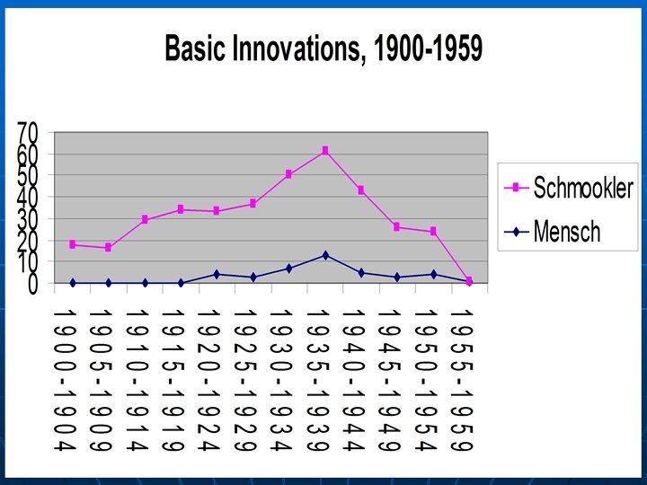
Sectoral Evidence n n R and D employment in manufacturing Time path of key innovations • • • n n Kleinknecht Schmookler Mensch MFP growth in telephone, railroads, electric utilities Build out of surface road system: network effects – impact on productivity growth in trucking and warehousing

R and D employment in US Manufacturing n n n 1927: 1933: 1940: 6, 274 10, 918 27, 777 Source: National Research Council data; Mowery and Rosenberg, 2000

Kleinknecht (1987)

The Irony of Secular Stagnation n At precisely the moment when Alvin Hansen and others were developing theories of secular stagnation, the U. S. economy was experiencing its greatest technological efflorescence, a period of creativity which, in the aggregate, remains unmatched to this day. His Harvard colleague, Joseph Schumpeter had a better fix on what was going on, although he misjudged the terrain on the road to socialism. Schumpeter’s homage to “creative destruction” was developed against the backdrop of what in fact has turned out to be the most technologically dynamic epoch of the twentieth century.

CAAGR of MFP, 1919 -1948 Telephone Electric Utilities 1919 -1929 1. 60% 1929 -1941 2. 01% 1941 -1948 0. 53% 2. 51% 5. 55% 5. 87% Railroads 1. 63% 2. 91% 2. 56%

Table 4: Compound Annual Average Growth Rates of Net Stock of Street and Highway Capital, United States, 1925 -2000 n n n 1925 -1929 -1941 -1948 -1973 -2000 6. 00% 4. 32% 0. 08% 4. 15% 1. 63%

Street/Highway Capital as % of Private Fixed Capital Street/Hway K Private Fixed K n n n 1929 $16, 415 $253, 987 1941 $30, 861 $289, 487 1948 $47, 892 $582, 248 1973 $290, 389 $2, 698, 194 2000 $1, 423, 833 $21, 464, 786 6. 46% 10. 66% 8. 22% 10. 76% 6. 63%

Two Waves of Government Investment: the 1930 and the 1940 s n n n Both decades experienced substantial government investment in physical capital 1930 s: Infrastructure 1940 s: Over $10 billion of GOPO capital in manufacturing, much of it equipment, especially machine tools The 1930 s investment generated spillovers that augmented PNE MFP growth, particularly in trucking and warehousing, and, through complementarities, in railroads. The 1940 s investment was associated with declining MFP growth in manufacturing and for the economy as a whole. What does this imply for the generality of the equipment hypothesis?

Summary – Field (2003) n n The 1930 s were characterized by productivity advance across a broad frontier of the U. S. economy. The expansion of potential output between 1919 and 1941 laid the foundation for postwar prosperity, at the same time that it enabled successful prosecution of the war. In the light of this finding we need to rethink our understanding of the defining contours and determinants of U. S. economic growth in the twentieth century.

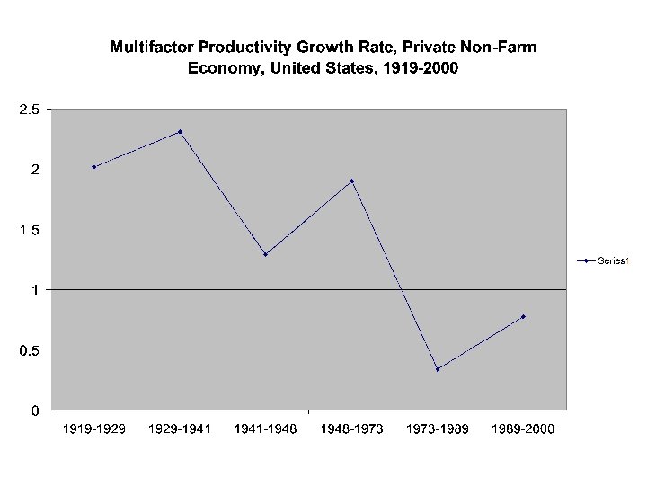
Field (2004) n n n Compares 1929 -41 with 1919 -29 on the one hand, and 1995 -2000 on the other Disaggregates, by broad sector, contributions to MFP growth in these different periods Reassesses IT’s impact on economic growth in the 1990 s, as well as the broader utility of the GPT concept with which it is closely associated.

Main Arguments n n MFP Growth in the 1920 s was almost entirely a story about manufacturing In the 1930 s, manufacturing’s contribution declined, although remaining high in absolute terms. Transport and Public Utilities played a much more important role. The same was true to a lesser extent of distribution. Although MFP growth between 1995 and 2000 was triple what it had been during 1973 -95, it was less than half what it was between 1929 and 1941. The IT revolution was responsible for about two thirds of MFP growth, and about a third of labor productivity growth between 1995 and 2000

CAAGR of MFP, PNE, United States, 1919 -2000 1919 -1929 -1941 -1948 -1973 -1989 -2000 2. 02 2. 31 1. 29 1. 90. 34. 78 1973 -1995 -2000 . 38 1. 14 Sources: 1919 -48: Field (2003); Kendrick (1961) 1948 -2000: Bureau of Labor Statistics: www. bls. gov

CAAGR of Labor Productivity, United States, 1919 -2000 1919 -1929 -1941 -1948 -1973 -1989 -2000 2. 27 2. 35 1. 71 2. 88 1. 33 1. 97 1973 -1995 -2000 1. 40 2. 43 Sources: 1919 -48: Kendrick (1961), Table A-23. 1948 -2000: Bureau of Labor Statistics: www. bls. gov

Labor Productivity Growth n n n Roughly comparable over 1919 -29, 192941, and 1995 -2000. The 1930 s were exceptional because advance took place in the virtual absence of capital deepening The 1948 -73 period remains the golden age of living standard improvement, because of the combined effects of respectable MFP growth and robust rates of capital deepening.

Labor Quality - 1 n n n How much of the growth in output per hour between 192941 is attributable to labor quality improvement? Margo (1991, 1993) has emphasized selective retention of higher quality workers as employment drops in a recession Not relevant for peak to peak comparisons; these composition effects would have been unwound as economy returned to full employment 1941 is much closer to full employment than 1940 or 1937, but still had 9. 9 percent unemployment, vs. less than 4 percent in 1929 In retrospect it would have been helpful for my research had Japan delayed attack on Pearl Harbor for another 8 to 12 months, so the U. S. economy could have continued its then rapid movement toward full employment before full scale war mobilization took place

Labor Quality 2 n n n Goldin (1998) has emphasized rapid rise in high school graduation rates in the 1930 s. R and D employment data for manufacturing and Margo’s analyses reflect strong demand for managerial, scientific, and technical personnel during this period Opportunity cost of high school attendance dropped as probability of a non high school grad being unemployed rose Build out of surface road network facilitated high school attendance Influx of human capital fleeing Hitler’s Europe

Labor Quality 3 n n n Labor Quality did rise between 1929 and 1941, but changes in labor supply were probably not a major or dominant influence on growth in output per hour If we calculate rate of growth of output per hour between 1929 -41 using adjusted hours, where adjusted hours take into account labor quality improvement, increase in output per hour is 6 percent less If selective retention were the dominant influence on growth as we came out of recession, we should have had a larger increment to output per hour moving from 19. 1 to 14. 6 percent unemployment between 1938 and 1940 than we did moving from 14. 6 to 9. 9 percent unemployment 1940 to 1941. But the reverse was true.

1929 -41 Manufacturing MFP Calculation n n Output: Hours: Capital: MFP: 3. 81 1. 35. 85 2. 60 percent/year Hours and output data from Kendrick; capital input data from BEA Fixed Asset Table 4. 2

1941 -48 Manufacturing MFP Calculation n n Output: Hours: Capital: MFP: 2. 20 percent/year 2. 17 percent/year 4. 02 percent/year -. 52 percent/year Hours and output data from Kendrick; capital input data from BEA Fixed Asset Table 4. 2

CAAGR of MFP, Manufacturing, United States, 1919 -2000 1919 -1929 -1941 -1948 -1973 -1995 -2000 5. 12 2. 60 -. 87 1. 52. 66 2. 09 Sources: Field (2004), Kendrick, (1961); Bureau of Economic Analysis Fixed Asset Table 4. 2; Bureau of Labor Statistics, Series MPU 300003 (B).

Manufacturing, 1919 -1929 n Share of PNE (1929): CAAGR, MFP(1919 -29): Cont to PNE MFP Growth: PNE MFP Growth (1919 -29): n Manufacturing’s Share: n n n . 333 5. 12% 1. 71% 2. 01% 85%

MFP Growth, Durable Manufacturing 19191929 Manufacturing Durable goods. . . . 5. 12 5. 06 19291948 194919732000 197319952000 1. 71 1. 52 0. 93 0. 66 2. 09 1. 43 1. 48 1. 57 1. 19 3. 27 Lumber and wood products. . . . . 2. 49 1. 42 1. 67 0. 65 0. 98 -0. 78 Furniture and fixtures. . . 4. 14 2. 00 0. 60 0. 74 0. 69 0. 96 Stone, clay, and glass products. . . 5. 57 2. 09 1. 09 0. 51 0. 49 0. 57 Primary metal industries. . . . . 5. 36 1. 30 0. 39 -0. 12 -0. 36 0. 95 Fabricated metal products. . . . . 4. 51 1. 36 0. 54 0. 20 0. 19 0. 26 Industrial, Commercial Machinery 2. 82 1. 62 0. 71 2. 93 2. 31 5. 65 Electric and electronic equipment. . . 3. 45 2. 55 2. 07 3. 85 3. 09 7. 18 Transport Equipment 8. 07 0. 39 1. 47 0. 18 0. 05 0. 72 4. 47* 2. 36* 1. 75 0. 97 1. 07 0. 54 1. 55 0. 47 0. 33 1. 10 Instruments and related products. . . Miscellaneous manufacturing. . . .

MFP Growth, Non. Durable Manufacturing 1919 -29 Nondurable goods. . . . 4. 89 1929 -48 2. 22 1949 -73 1973 -2000 1973 -95 1995 -2000 1. 32 0. 14 0. 06 0. 47 Food and kindred products. . . . . 5. 18 1. 47 0. 67 0. 26 0. 39 -0. 31 Tobacco products. . . . 4. 28 4. 19 -0. 62 -3. 71 -2. 92 -7. 19 Textile mill products. . . 2. 90 3. 28 2. 29 2. 23 2. 32 1. 87 Apparel and other textile products. . . 3. 90 0. 63 0. 72 1. 00 0. 91 1. 41 Paper and allied products. . . . . 4. 54 2. 33 1. 58 -0. 11 -0. 31 0. 74 Printing and publishing. . . . . 3. 67 1. 43 0. 48 -0. 73 -0. 94 0. 22 Chemicals and allied products. . . . 7. 15 3. 36 2. 51 -0. 25 -0. 42 0. 51 Petroleum and coal products. . . . 8. 23 1. 70 0. 82 0. 03 -0. 14 0. 77 Rubber and miscellaneous plastics products. . . 7. 40 2. 07 0. 96 0. 64 0. 42 1. 60 Leather and leather products. . . . 2. 88 1. 71 0. 02 0. 58 0. 21 2. 23

Manufacturing, 1929 -1941 n n n Share of PNE (1941): CAAGR, MFP (1929 -41): Cont to PNE MFP Growth: PNE MFP Growth (1929 -41): Manufacturing’s Share: . 426 2. 60% 1. 11% 2. 31% 48%

Manufacturing, 1995 -2000 n n n Share of PNE (2000): CAAGR, MFP(1995 -00): Cont to PNE MFP Growth: PNE MFP Growth (1995 -00): Manufacturing’s Share: . 214 2. 08%. 45% 1. 14% 39%

Transport and Public Utilities 19191929 n n n Share of PNE (1929): CAAGR, MFP(1919 -29): Cont to PNE MFP Growth: PNE MFP Growth (1919 -29): Sector’s Share: . 14 1. 86%. 27% 2. 01% 13%

Transport and Public Utilities 19291941 n n n Share of PNE (1941): CAAGR, MFP(1929 -41): Cont to PNE MFP Growth: PNE MFP Growth (1929 -41): Sector’s Share: . 123 4. 67%. 58% 2. 31% 25%

Transport and Public Utilities 19291941 n n n 26 percent of sector MFP growth comes from railroads 40 percent of sector MFP growth comes from trucking & warehousing 10 percent of total private non farm MFP growth comes from trucking & warehousing

Table 7 MFP Growth, Transportation and Public Utilities, 1929 -1941 1929 -41 Share of Subsector NI*100 of Covered MFP Contribution 1941(1948) T & PU Subsectors Growth MFP Growth Railroad transportation. . . . . 3. 27 0. 372 Local and interurban passenger transit. . 0. 66 0. 075 Trucking and warehousing. . . . . 1. 03 0. 117 Water transportation. . . 0. 42 0. 048 Transportation by air. . . 0. 18 0. 021 Pipelines, except natural gas. . . . 0. 10 0. 012 Transportation services. . . . . 0. 13 0. 014 Telephone and telegraph. . . . . 1. 30 0. 148 Radio and television. . . 0. 10 0. 011 Electric, gas, and sanitary services. . . 1. 61 0. 183 8. 81 TOTAL 0. 420 0. 084 0. 132 0. 054 0. 023 0. 013 2. 91 3. 02 13. 57 1. 47 14. 69 4. 48 1. 22 0. 25 1. 80 0. 08 0. 34 0. 06 0. 167 2. 02 0. 34 0. 104 0. 57 5. 55 4. 67

Wholesale and Retail Trade 1919 -1929 n n n Share of PNE (1929): . 201 CAAGR, MFP(1919 -29): . 80% Cont to PNE MFP Growth: . 17% PNE MFP Growth (1919 -29): 2. 01% Trade’s Share MFP Growth: 8%

Wholesale and Retail Trade 1929 -1941 n n n Share of PNE (1941): CAAGR, MFP(1929 -41): Cont to PNE MFP Growth: PNE MFP Growth (1929 -41): Trade’s Share MFP Growth: . 223 1. 81%. 40% 2. 31% 18%

Wholesale and Retail Trade 1995 -2000 n n n Share of PNE (2000): . 223 CAAGR, MFP(1995 -00): . 70 % Cont to PNE MFP Growth: . 16% PNE MFP Growth (1995 -00): 1. 14% Trade’s Share MFP Growth: 14 %

Let’s Remove Religion from the Analysis of Productivity Trends n n n Late 1990 s: New economy skeptics and true believers The move from skeptic to believer as a matter of “Getting Religion”; akin to a process of spiritual conversion Use of vignettes and anecdotes Is this really the way to discipline our conclusions with data? Focus on what the data actually reveal, rather than what they might reveal in the future, or we hope they will reveal in the future With the marked acceleration in both MFP and labor productivity growth 1995 -2000, one can no longer claim the statistical apparatus is incapable of picking up effects of IT.

Reckoning The Impact of IT on Labor Productivity Growth Conventional Framework: 3 parts 1. MFP growth within IT producing sector 2. MFP growth within IT using sectors (spillovers) 3. That portion of the impact of capital deepening on labor productivity growth associated with the accumulation of IT capital goods

Why Include the Third Component? n n n In the absence of IT, saving flows would have been congealed in a slightly inferior range of capital goods. Social Savings Analogy. Debate between Rostow on the one hand Fishlow and Fogel on the other. Fogel and Fishlow imagined worlds in all respects similar save the availability of railway technology. Fogel: Because of the railroad, GDP was higher in 1890. But not that much higher: the availability of the technology made a difference of 4 percent Over a 25 year period, what kind of an annual increment to MFP growth does one need to produce a 4 percent increase in GDP? . 15 percentage points In MFP terms, that’s the railroad’s contribution

Rostow Redux n Would it be reasonable for supporters of the “indispensability” thesis to object that Fogel’s estimate vastly underestimated the contribution of the railroad to labor productivity growth and US standards of living because it failed to take into account that portion of labor productivity growth attributable to the (substantial) fraction of capital deepening associated with the accumulation of railway permanent way, bridges, tunnels, roundtables, stations, locomotives, and rolling stock?

Solow Again n n It remains worthwhile distinguishing between the effects on labor productivity of thrift and innovation There is little evidence that saving rates accelerated in the presence of the IT revolution

Sources and Uses of Saving S = I + (G-T) + (X-M) Private Domestic Saving funds Private Domestic Capital Accumulation, the Government Deficit, and capital accumulation outside of the Country I = S + (T-G) + (M-X) Private Domestic Capital Accumulation must be funded by the sum of private domestic saving, government saving, and the capital account surplus (inflows of foreign saving).

End of Century Tangible Capital Accumulation n n Whatever one can say about the rising importance of human capital formation in the twentieth century, a distinguishing feature of the 1995 -2000 was a rise in tangible capital accumulation, with a heavy emphasis on short lived equipment. Capital services growth accelerated from 3. 94 percent per year (1973 -95) to 5. 38 percent per year (1995 -2000). The capital deepening that made this possible required capital accumulation that had to be financed. As growth of IT capital services accelerated from. 41 to 1. 03 percent per year, growth of non IT capital services essentially halted, dropping from. 30 to. 06 percent per year. Inflow of foreign saving represented a slowing of capital services growth outside of the country.

Sources and Uses of Saving, US, 1995 -2000 1995 2000 1, 143. 8 238. 2 1, 755. 4 319. 8 302. 4 203. 6 743. 6 963. 6 201. 5 152. 6 1, 017. 9 1, 170. 5 -100. 9 206. 9 Gross Government Saving -8. 5 435. 8 444. 3 Capital Account Surplus 98. 0 395. 8 297. 8 Statistical Discrepancy 26. 5 -128. 5 -155. 0 Gross Private Domestic Investment Gross Government Investment Personal Saving Retained Business Earnings Depreciation Allowances Gross Business Saving* TOTALS Change in uses Change in sources 611. 6 81. 6 693. 2 693. 1

Table 13 MFP Contribution to Labor Productivity Growth and Acceleration, 1995 -2000 Labor Productivity Growth, 1995 -2000 a 2. 46 MFP a 1. 14 Capital deepening a 1. 05 Labor Composition a . 26 Labor Productivity Growth Acceleration, 1995 -2000 vs. 1973 -95 b 1. 09 MFP b . 76 Capital Deepening b . 32 Labor Composition b -. 01 a percent per year percentage points Note: Components do not sum exactly to aggregates due to rounding errors. b

Table 16 Sectoral Contributions to MFP growth, 1995 -2000 Share of PNE Sectoral MFP Growth Contribution to PNE MFP Growth Share of PNE MFP Growth Manufacturing . 214 2. 08 . 45. 39 Trade . 223 . 70 . 16. 14 Other . 563 . 94 . 53. 47 TOTAL 1. 00 1. 14 Sources: Sectoral Shares: see Table 3 Note: Private Nonfarm economy excludes nonfarm housing, health, agriculture, and government, which leaves 72. 4 percent of value added. MFP growth Manufacturing: see Table 5 MFP growth Trade: see text

IT’s Contribution n n Credit IT with all MFP growth in Manufacturing Credit IT with one third of MFP growth in the rest of the economy. 68 of 1. 14 percent per year (about 60 percent) of MFP growth between 1995 and 2000 attributable to IT 28 percent of labor productivity growth 1995 -2000 is attributable to the IT revolution (. 68/2. 46 percent per year)

The Equipment Hypothesis n De Long and Summers (1991) • Cross country regressions using 1960 -85 data show a relationship between share of equipment investment in GDP and the growth of output per worker n Auerbach, Hasset, and Oliner (1994) • Criticize econometrics, question whether conclusion is applicable to US n Field (2004) • The drop in relative prices of equipment, and increase in equipment’s share of capital formation in the US coincides with a long term decline in the rate of MFP advance from its high rates in the interwar period to its virtual disappearance in the last quarter of the century • Is 1995 -2000 an aberration, or a fundamental turning point in US. productivity history?

GPT’s n n n Distinguish between the proposition that it sometimes takes a long time for the productivity benefits of new technological complexes to be reaped, and the usefulness of the concept of a GPT Potential multiplicity of candidates: Steam, electricity, IT are most frequently identified, but chemical engineering, the internal combustion engine, radio transmission and the assembly line have also been mentioned. Identification of one or several GPT’s often offers an appealing narrative hook, but the criteria for designating them are not universally agreed upon, in spite of continuing efforts to nail them down. Why isn’t the railroad also a GPT? Gordon (2004) suggests that use by both households and industry is a criterion. This works for electricity and the internal combustion engine. But steam?

GPTs n Bessemer and Siemens Martin processes were industry specific, and would clearly not pass muster as GPTs. They offered, to use David’s words, “complete, self-contained and immediately applicable solutions. ” This was not the case for the product whose production they enabled. Does that make steel a GPT? It took Carnegie and others time to persuade users they should make skyscrapers, plate ships, and replace rails with it. Cheap steel in turn encouraged complementary innovations such as, in the case of taller buildings, elevators.

GPTs n n If one follows the impact of product and process innovations far enough through the input-output table, one will eventually find products or technological complexes used as inputs in many other sectors, with the potential to generate spillover effects in using sectors. These processes, products, or complexes are the consequence of many separate breakthroughs as well as learning by doing, much of which has been sector specific. IT for example, has required advances in sector specific semiconductor manufacturing, and the thin film technology and mechanical engineering that underlies most mass storage, let alone software. Because of the potential for multiplying GPT candidacies and the lack of an authoritative tribunal applying uniform rules passing judgment about which ones qualify, economic and technological history may be better off without the concept.

Conclusions n IT was responsible for about 60 percent of MFP growth and about 28 percent of labor productivity growth between 1995 and 2000

Conclusions n n n MFP Growth in the 1920 s was 15 percent lower than the benchmark 1929 -41 period. During the 1920 s it was almost entirely a story about progress in manufacturing, although advance was broadly experienced throughout the sector, in contrast with the 1990 s In the 1930 s, manufacturing’s contribution declined, although remaining high in absolute terms. Transport and Public Utilities played a much more important role. The same was true to a lesser extent of distribution. These latter effects reflect a roughly three decade long delay between the invention of the internal combustion engine and the full reaping of its productivity benefits in using sectors. MFP growth in 1995 -2000 was three times what it had been during the anemic years 1973 -1995, but less than half the rate clocked between 1929 and 1941.

Conclusions n n n In accounting for the expansion of potential output, there is no single process, product, or technological complex for the 1930 s around which one can build a compelling narrative. What was exceptional about 1929 -41, distinguishing the period from the other two examined in this paper, was the broad frontier across which technological progress was advancing. In contrast, MFP advance 1995 -2000 was narrowly concentrated within a declining manufacturing sector in SIC 35 and 36, and within the using sectors in wholesale and retail trade and securities trading.

A Century of Technological Expositions n 1893 –Chicago • Columbian Exposition – The White City • AC current for illumination, but still powered by coal and steam n 1939 -40 – New York • GM’s Futurama – Norman Bel Geddes’ wildly popular and largely accurate vision of the US in 1960 • Democracity n 1964 -65 – New York • Failure of the new Futurama – either to inspire or to accurately forecast n 1996 – Anaheim • A Retro Tomorrowland

Is Comdex a Substitute? n n n The last “successful” North American world’s fair was Expo ’ 67 at Montreal, and the first (and last Asian fair Expo ’ 70 was also a success Subsequent fairs (Spokane - 1974, Knoxville - 1982, New Orleans - 1984, Vancouver - 1986, and Seville -1992) have been more narrowly themed. Who now remembers them? The fading impact of these international expositions coincides roughly with the collapse of the residual beginning in the 1970 s. World’s fairs emerged out of commercial fairs, and in the 1990 s trade shows such as Comdex generated some of the same kind of excitement as had earlier international expositions, but they were much more narrowly focused, reflecting the relatively narrow based of technical advance in recent years, and have not been targeted at the general public.

Table 9 Sectoral Contributions to Multifactor Productivity Growth Within the Private Nonfarm Economy United States, 1929 -1941 Sectoral Manufacturing Transport and Public Utilities Wholesale and Retail Trade Other Sectors (net) Mining Construction Finance, Insurance, Real Estate (see note a) Other Services (see note b) TOTAL 1941 Share of Private National Income Nonfarm Economy MFP Growth 1929 -1941 Sector's Contribution to Aggregate (PNE) MFP Growth 31. 86 9. 21 16. 70 42. 57 12. 30 22. 31 2. 91 4. 48 1. 81 1. 239 0. 551 0. 404 17. 08 22. 82 0. 51 0. 116 2. 30 4. 03 4. 78 5. 97 74. 85 100. 00 2. 310