TAMPERE UNIVERSITY OF TECHNOLOGY TELETRAFFIC THEORY PART 1

TAMPERE UNIVERSITY OF TECHNOLOGY TELETRAFFIC THEORY (PART 1) Exercises #1 Andrey Krendzel krendzel@cs. tut. fi www. cs. tut. fi/kurssit/8303700

EXERSISES 1 Reminder of Probability Theory CONTENTS 1. Sets and Probability 1. 1 Sets and Subsets 1. 2 Set Operations 1. 3 Sample Space 1. 4 Techniques of Counting 1. 5 Probability 1. 6 Conditional Probability 1. 7 Bayes’ Theorem 2. Random Variables 2. 1 Discrete Random Variables 2. 2 Continuous Random Variables 2. 3 Normal Distribution 2. 4 Poisson Distribution

EXERSISES 1 Reminder of Probability Theory 1. 1 Sets and Subsets Example Let A = {2, 4, 6, 8} and B = {x| x is an integer divisible by 3}. Then 4 A, 9 B, 8 B, and 3 A. Definition Two sets are equal if they have exactly the same elements in them. Example Let A = {1, 3, 5}, B = {3, 1, 5}, and C = {1, 3, 5, 7}. Then = B, A C, and B C. Definition The null set or empty set is a set that contains no elements. We denote this set by the symbol . Definition If every element of a set A is also an element of a set B, then A is called a subset of B, A B. Problem 1 Find all the subsets of the set U = {1, 2, 3} A

EXERSISES 1 Reminder of Probability Theory Problem 1 All the subsets of the set U = {1, 2, 3}, are {1, 2, 3}, {1, 2}, {1, 3}, {2, 3}, {1}, {2}, {3}, { }.

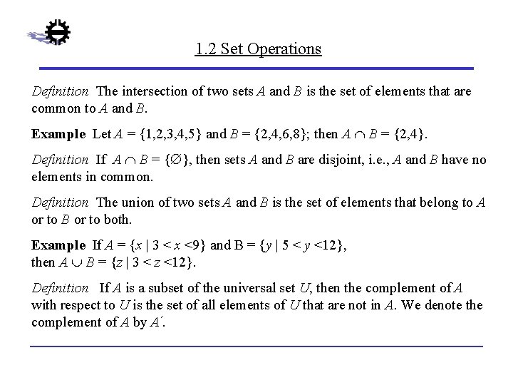
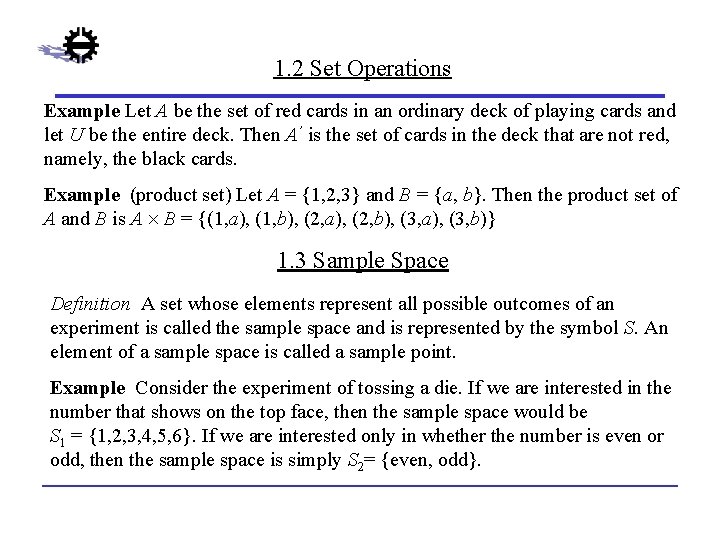
1. 2 Set Operations Definition The intersection of two sets A and B is the set of elements that are common to A and B. Example Let A = {1, 2, 3, 4, 5} and B = {2, 4, 6, 8}; then A B = {2, 4}. Definition If A B = { }, then sets A and B are disjoint, i. e. , A and B have no elements in common. Definition The union of two sets A and B is the set of elements that belong to A or to B or to both. Example If A = {x | 3 < x <9} and B = {y | 5 < y <12}, then A B = {z | 3 < z <12}. Definition If A is a subset of the universal set U, then the complement of A with respect to U is the set of all elements of U that are not in A. We denote the complement of A by A’.

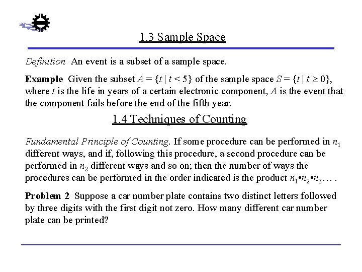
1. 2 Set Operations Example Let A be the set of red cards in an ordinary deck of playing cards and let U be the entire deck. Then A’ is the set of cards in the deck that are not red, namely, the black cards. Example (product set) Let A = {1, 2, 3} and B = {a, b}. Then the product set of A and B is A B = {(1, a), (1, b), (2, a), (2, b), (3, a), (3, b)} 1. 3 Sample Space Definition A set whose elements represent all possible outcomes of an experiment is called the sample space and is represented by the symbol S. An element of a sample space is called a sample point. Example Consider the experiment of tossing a die. If we are interested in the number that shows on the top face, then the sample space would be S 1 = {1, 2, 3, 4, 5, 6}. If we are interested only in whether the number is even or odd, then the sample space is simply S 2= {even, odd}.

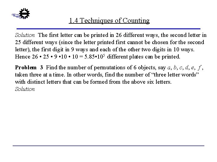
1. 3 Sample Space Definition An event is a subset of a sample space. Example Given the subset A = {t | t < 5} of the sample space S = {t | t 0}, where t is the life in years of a certain electronic component, A is the event that the component fails before the end of the fifth year. 1. 4 Techniques of Counting Fundamental Principle of Counting. If some procedure can be performed in n 1 different ways, and if, following this procedure, a second procedure can be performed in n 2 different ways and so on; then the number of ways the procedures can be performed in the order indicated is the product n 1 • n 2 • n 3…. Problem 2 Suppose a car number plate contains two distinct letters followed by three digits with the first digit not zero. How many different car number plate can be printed?

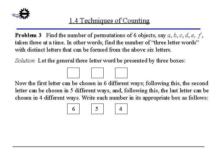
1. 4 Techniques of Counting Solution The first letter can be printed in 26 different ways, the second letter in 25 different ways (since the letter printed first cannot be chosen for the second letter), the first digit in 9 ways and each of the other two digits in 10 ways. Hence 26 • 25 • 9 • 10 = 5. 85 • 105 different plates can be printed. Problem 3 Find the number of permutations of 6 objects, say a, b, c, d, e, f , taken three at a time. In other words, find the number of “three letter words” with distinct letters that can be formed from the above six letters. Solution

1. 4 Techniques of Counting Problem 3 Find the number of permutations of 6 objects, say a, b, c, d, e, f , taken three at a time. In other words, find the number of “three letter words” with distinct letters that can be formed from the above six letters. Solution Let the general three letter word be presented by three boxes: Now the first letter can be chosen in 6 different ways; following this, the second letter can be chosen in 5 different ways, and, following this, the last letter can be chosen in 4 different ways. Write each number in its appropriate box as follows: 6 5 4

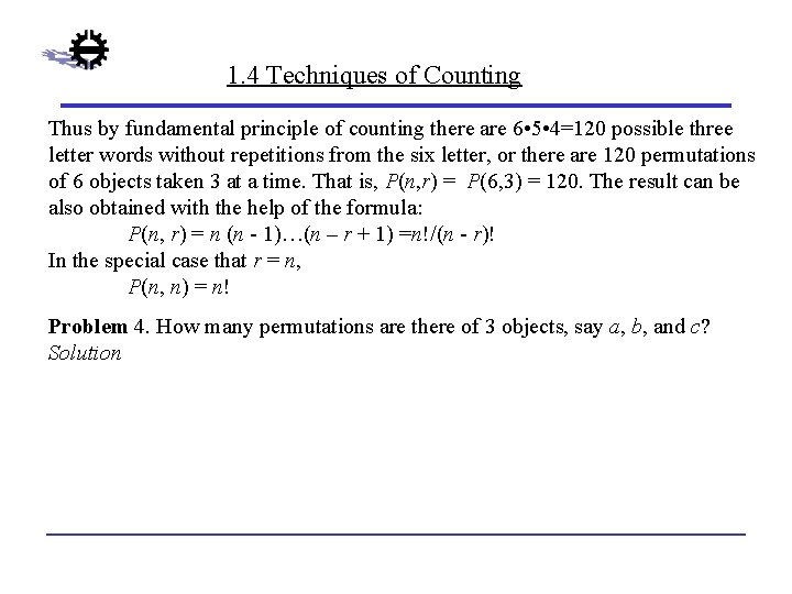
1. 4 Techniques of Counting Thus by fundamental principle of counting there are 6 • 5 • 4=120 possible three letter words without repetitions from the six letter, or there are 120 permutations of 6 objects taken 3 at a time. That is, P(n, r) = P(6, 3) = 120. The result can be also obtained with the help of the formula: P(n, r) = n (n - 1)…(n – r + 1) =n!/(n - r)! In the special case that r = n, P(n, n) = n! Problem 4. How many permutations are there of 3 objects, say a, b, and c? Solution

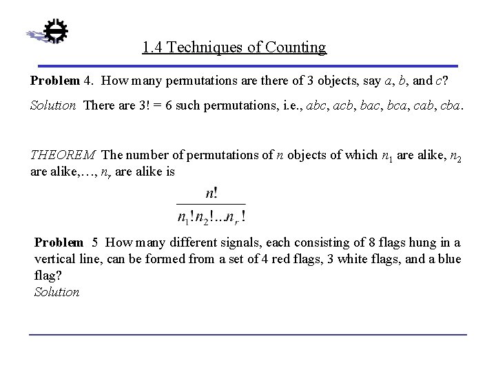
1. 4 Techniques of Counting Problem 4. How many permutations are there of 3 objects, say a, b, and c? Solution There are 3! = 6 such permutations, i. e. , abc, acb, bac, bca, cab, cba. THEOREM The number of permutations of n objects of which n 1 are alike, n 2 are alike, …, nr are alike is Problem 5 How many different signals, each consisting of 8 flags hung in a vertical line, can be formed from a set of 4 red flags, 3 white flags, and a blue flag? Solution

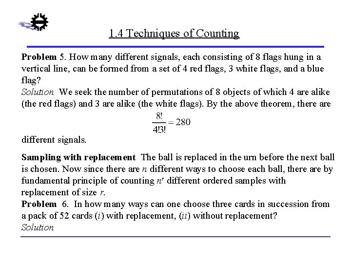
1. 4 Techniques of Counting Problem 5. How many different signals, each consisting of 8 flags hung in a vertical line, can be formed from a set of 4 red flags, 3 white flags, and a blue flag? Solution We seek the number of permutations of 8 objects of which 4 are alike (the red flags) and 3 are alike (the white flags). By the above theorem, there are different signals. Sampling with replacement The ball is replaced in the urn before the next ball is chosen. Now since there are n different ways to choose each ball, there are by fundamental principle of counting nr different ordered samples with replacement of size r. Problem 6. In how many ways can one choose three cards in succession from a pack of 52 cards (i) with replacement, (ii) without replacement? Solution

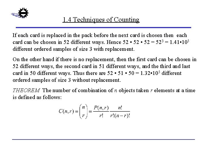
1. 4 Techniques of Counting If each card is replaced in the pack before the next card is chosen then each card can be chosen in 52 different ways. Hence 52 • 52 = 523 = 1. 41 • 105 different ordered samples of size 3 with replacement. On the other hand if there is no replacement, then the first card can be chosen in 52 different ways, the second card in 51 different ways, and the third and last card in 50 different ways. Thus there are 52 • 51 • 50 = 1. 32 • 105 different ordered samples of size 3 without replacement. THEOREM The number of combination of n objects taken r elements at a time is defined as follows:

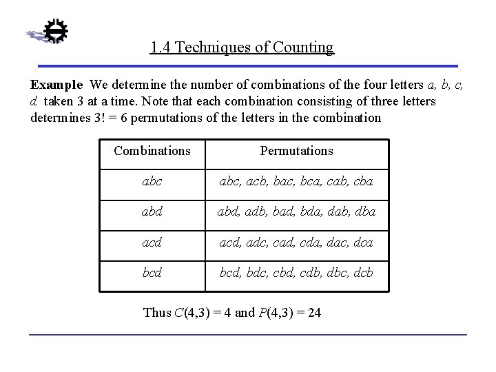
1. 4 Techniques of Counting Example We determine the number of combinations of the four letters a, b, c, d taken 3 at a time. Note that each combination consisting of three letters determines 3! = 6 permutations of the letters in the combination Combinations Permutations abc, acb, bac, bca, cab, cba abd, adb, bad, bda, dab, dba acd, adc, cad, cda, dac, dca bcd, bdc, cbd, cdb, dbc, dcb Thus C(4, 3) = 4 and P(4, 3) = 24

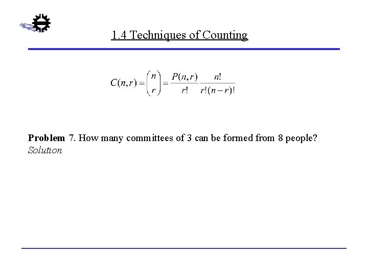
1. 4 Techniques of Counting Problem 7. How many committees of 3 can be formed from 8 people? Solution

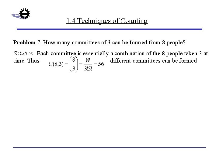
1. 4 Techniques of Counting Problem 7. How many committees of 3 can be formed from 8 people? Solution Each committee is essentially a combination of the 8 people taken 3 at time. Thus different committees can be formed

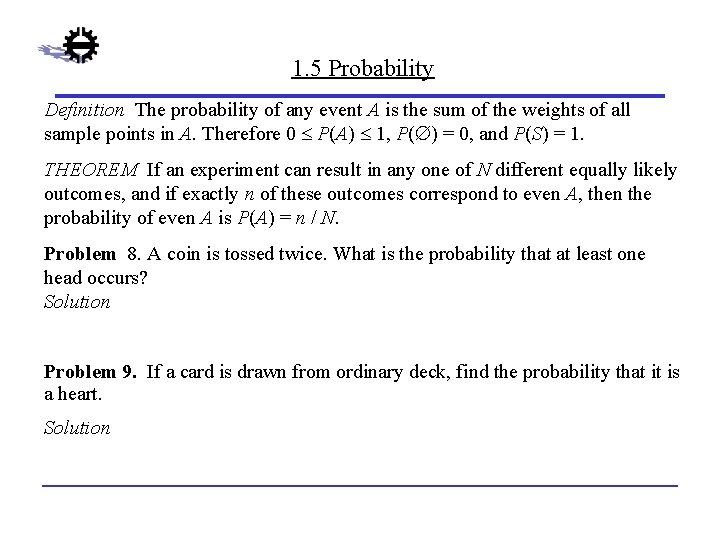
1. 5 Probability Definition The probability of any event A is the sum of the weights of all sample points in A. Therefore 0 P(A) 1, P( ) = 0, and P(S) = 1. THEOREM If an experiment can result in any one of N different equally likely outcomes, and if exactly n of these outcomes correspond to even A, then the probability of even A is P(A) = n / N. Problem 8. A coin is tossed twice. What is the probability that at least one head occurs? Solution Problem 9. If a card is drawn from ordinary deck, find the probability that it is a heart. Solution

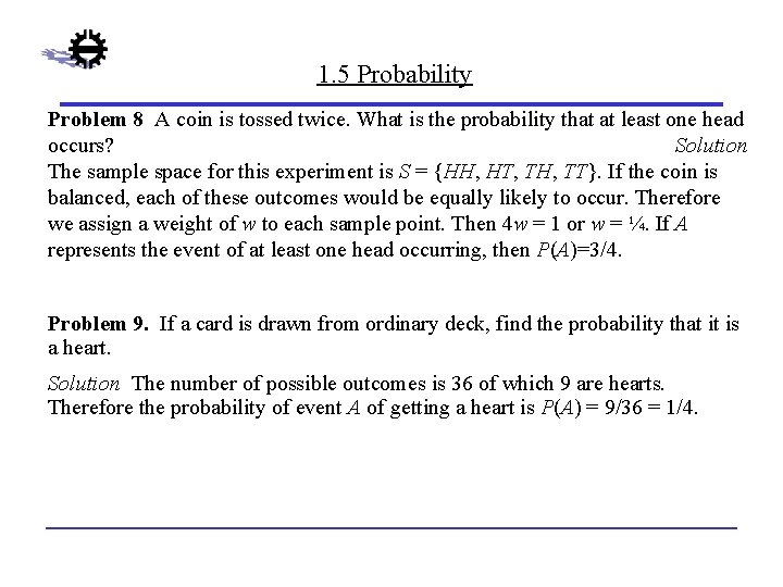
1. 5 Probability Problem 8 A coin is tossed twice. What is the probability that at least one head occurs? Solution The sample space for this experiment is S = {HH, HT, TH, TT}. If the coin is balanced, each of these outcomes would be equally likely to occur. Therefore we assign a weight of w to each sample point. Then 4 w = 1 or w = ¼. If A represents the event of at least one head occurring, then P(A)=3/4. Problem 9. If a card is drawn from ordinary deck, find the probability that it is a heart. Solution The number of possible outcomes is 36 of which 9 are hearts. Therefore the probability of event A of getting a heart is P(A) = 9/36 = 1/4.

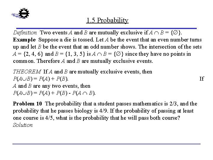
1. 5 Probability Definition Two events A and B are mutually exclusive if A B = { }. Example Suppose a die is tossed. Let A be the event that an even number turns up and let B be the event that an odd number shows. The intersection of the sets A = {2, 4, 6} and B = {1, 3, 5} is A B = { } since they have no points in common. Therefore A and B are mutually exclusive events. THEOREM If A and B are mutually exclusive events, then P(A B) = P(A) + P(B). A and B are any two events, then P(A B) = P(A) + P(B) - P(A B). Problem 10 The probability that a student passes mathematics is 2/3, and the probability that he passes biology is 4/9. If the probability of passing at least one course is 4/5, what is the probability that he will pass both course? Solution If

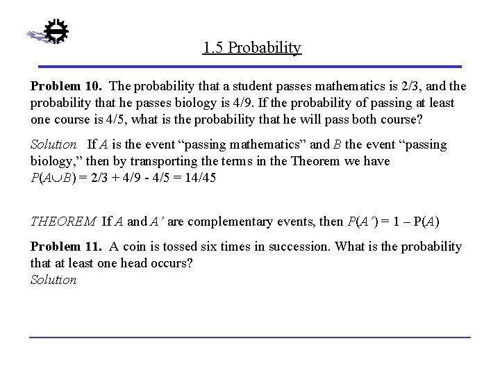
1. 5 Probability Problem 10. The probability that a student passes mathematics is 2/3, and the probability that he passes biology is 4/9. If the probability of passing at least one course is 4/5, what is the probability that he will pass both course? Solution If A is the event “passing mathematics” and B the event “passing biology, ” then by transporting the terms in the Theorem we have P(A B) = 2/3 + 4/9 - 4/5 = 14/45 THEOREM If A and A’ are complementary events, then P(A’) = 1 – P(A) Problem 11. A coin is tossed six times in succession. What is the probability that at least one head occurs? Solution

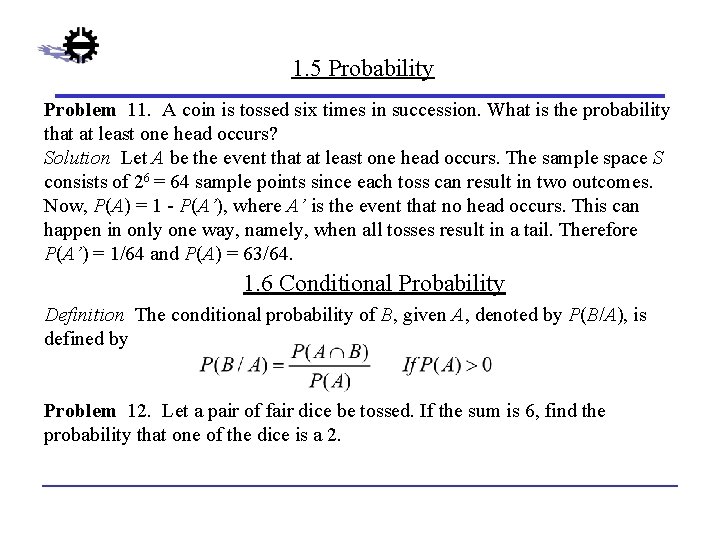
1. 5 Probability Problem 11. A coin is tossed six times in succession. What is the probability that at least one head occurs? Solution Let A be the event that at least one head occurs. The sample space S consists of 26 = 64 sample points since each toss can result in two outcomes. Now, P(A) = 1 - P(A’), where A’ is the event that no head occurs. This can happen in only one way, namely, when all tosses result in a tail. Therefore P(A’) = 1/64 and P(A) = 63/64. 1. 6 Conditional Probability Definition The conditional probability of B, given A, denoted by P(B/A), is defined by Problem 12. Let a pair of fair dice be tossed. If the sum is 6, find the probability that one of the dice is a 2.

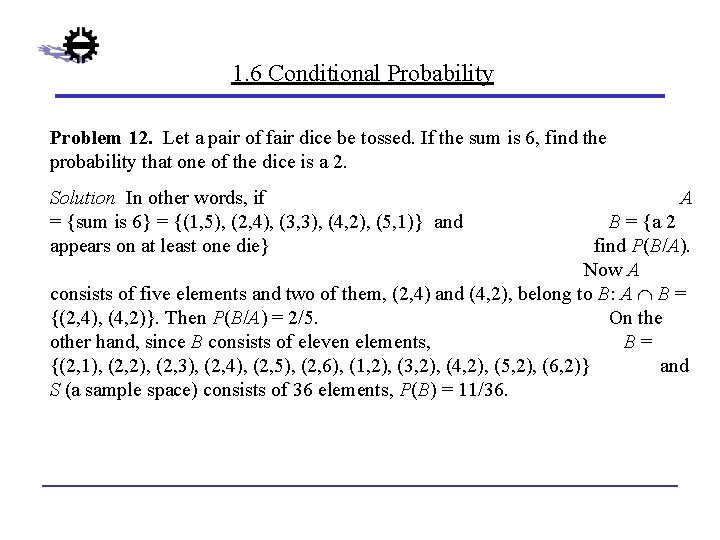
1. 6 Conditional Probability Problem 12. Let a pair of fair dice be tossed. If the sum is 6, find the probability that one of the dice is a 2. Solution In other words, if = {sum is 6} = {(1, 5), (2, 4), (3, 3), (4, 2), (5, 1)} and appears on at least one die} A B = {a 2 find P(B/A). Now A consists of five elements and two of them, (2, 4) and (4, 2), belong to B: A B = {(2, 4), (4, 2)}. Then P(B/A) = 2/5. On the other hand, since B consists of eleven elements, B= {(2, 1), (2, 2), (2, 3), (2, 4), (2, 5), (2, 6), (1, 2), (3, 2), (4, 2), (5, 2), (6, 2)} and S (a sample space) consists of 36 elements, P(B) = 11/36.

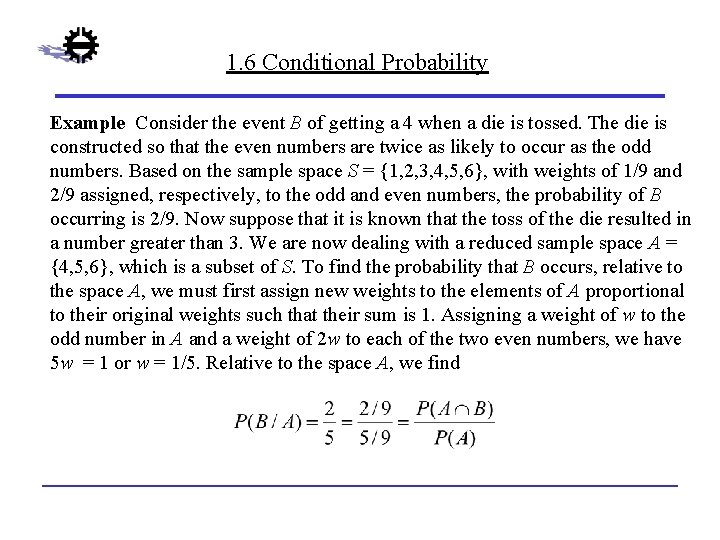
1. 6 Conditional Probability Example Consider the event B of getting a 4 when a die is tossed. The die is constructed so that the even numbers are twice as likely to occur as the odd numbers. Based on the sample space S = {1, 2, 3, 4, 5, 6}, with weights of 1/9 and 2/9 assigned, respectively, to the odd and even numbers, the probability of B occurring is 2/9. Now suppose that it is known that the toss of the die resulted in a number greater than 3. We are now dealing with a reduced sample space A = {4, 5, 6}, which is a subset of S. To find the probability that B occurs, relative to the space A, we must first assign new weights to the elements of A proportional to their original weights such that their sum is 1. Assigning a weight of w to the odd number in A and a weight of 2 w to each of the two even numbers, we have 5 w = 1 or w = 1/5. Relative to the space A, we find

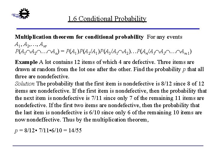
1. 6 Conditional Probability Multiplication theorem for conditional probability For any events A 1, A 2, …, An, P(A 1 A 2 … An) = P(A 1)P(A 2/A 1)P(A 3/A 1 A 2)…P(An/A 1 A 2 … An-1) Example A lot contains 12 items of which 4 are defective. Three items are drawn at random from the lot one after the other. Find the probability p that all three are nondefective. Solution The probability that the first item is nondefective is 8/12 since 8 of 12 items are nondefective. If the first item is nondefective, then the probability that the next item is nondefective is 7/11 since only 7 of the remaining 11 items are nondefective. If the first two items are nondefective, then the probability that the last item is nondefective is 6/10 since only 6 of the remaining 10 items are now nondeffective. Thus by the multiplication theorem, p = 8/12 • 7/11 • 6/10 = 14/55

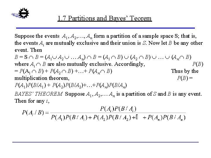
1. 7 Partitions and Bayes’ Teorem Suppose the events A 1, A 2, …, An form a partition of a sample space S; that is, the events Ai are mutually exclusive and their union is S. Now let B be any other event. Then B = S B = (A 1 A 2 … An) B = (A 1 B) (A 2 B) … (An B) where Ai B are also mutually exclusive. Accordingly, P(B) = P(A 1 B) + P(A 2 B) +…+ P(An B) Thus by the multiplication theorem, P(B) = P(A 1)P(B/A 1) + P(A 2)P(B/A 2)+…+P(An)P(B/An) BAYES’ THEOREM Suppose A 1, A 2, … An is a partition of S and B is any event. Then for any i,

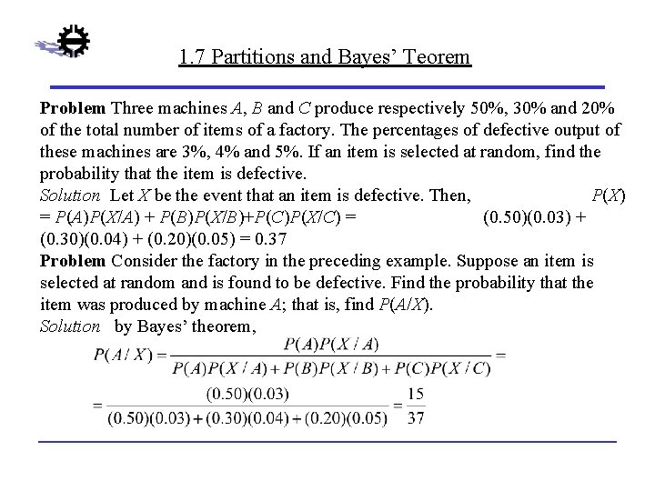
1. 7 Partitions and Bayes’ Teorem Problem Three machines A, B and C produce respectively 50%, 30% and 20% of the total number of items of a factory. The percentages of defective output of these machines are 3%, 4% and 5%. If an item is selected at random, find the probability that the item is defective. Solution Let X be the event that an item is defective. Then, P(X) = P(A)P(X/A) + P(B)P(X/B)+P(C)P(X/C) = (0. 50)(0. 03) + (0. 30)(0. 04) + (0. 20)(0. 05) = 0. 37 Problem Consider the factory in the preceding example. Suppose an item is selected at random and is found to be defective. Find the probability that the item was produced by machine A; that is, find P(A/X). Solution by Bayes’ theorem,

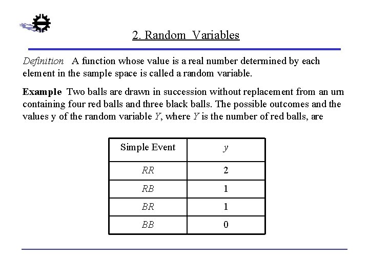
2. Random Variables Definition A function whose value is a real number determined by each element in the sample space is called a random variable. Example Two balls are drawn in succession without replacement from an urn containing four red balls and three black balls. The possible outcomes and the values y of the random variable Y, where Y is the number of red balls, are Simple Event y RR 2 RB 1 BR 1 BB 0

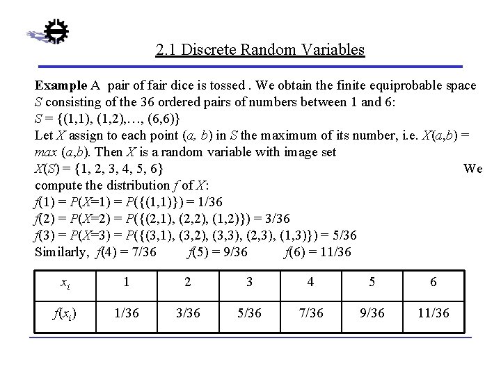
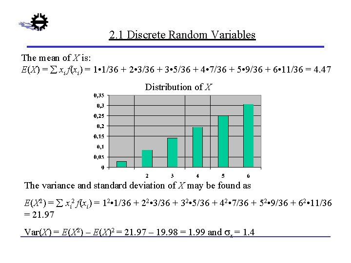
2. 1 Discrete Random Variables Example A pair of fair dice is tossed. We obtain the finite equiprobable space S consisting of the 36 ordered pairs of numbers between 1 and 6: S = {(1, 1), (1, 2), …, (6, 6)} Let X assign to each point (a, b) in S the maximum of its number, i. e. X(a, b) = max (a, b). Then X is a random variable with image set X(S) = {1, 2, 3, 4, 5, 6} We compute the distribution f of X: f(1) = P(X=1) = P({(1, 1)}) = 1/36 f(2) = P(X=2) = P({(2, 1), (2, 2), (1, 2)}) = 3/36 f(3) = P(X=3) = P({(3, 1), (3, 2), (3, 3), (2, 3), (1, 3)}) = 5/36 Similarly, f(4) = 7/36 f(5) = 9/36 f(6) = 11/36 xi 1 2 3 4 5 6 f(xi) 1/36 3/36 5/36 7/36 9/36 11/36

2. 1 Discrete Random Variables The mean of X is: E(X) = xi f(xi) = 1 • 1/36 + 2 • 3/36 + 3 • 5/36 + 4 • 7/36 + 5 • 9/36 + 6 • 11/36 = 4. 47 Distribution of X The variance and standard deviation of X may be found as E(X 2) = xi 2 f(xi) = 12 • 1/36 + 22 • 3/36 + 32 • 5/36 + 42 • 7/36 + 52 • 9/36 + 62 • 11/36 = 21. 97 Var(X) = E(X 2) – E(X)2 = 21. 97 – 19. 98 = 1. 99 and x = 1. 4

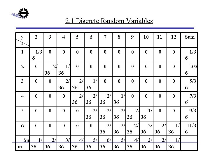
2. 1 Discrete Random Variables Joint Distribution Let X and Y be random variables on a sample space S with respective sets X(S) = {x 1, x 2, …, xn} and Y(S) = {y 1, y 2, …ym} We make the product set X(S)Y(S) = {(x 1 y 1), (x 2, y 2), …, (xn, ym)} into a probability space by defining the probability of the ordered pair h(xi, yi). This function h is called the joint distribution or joint probability function of X and Y and is usually given in the form of a table. Example A pair of fair dice is tossed. We obtain the finite equiprobable space consisting of the 36 ordered pairs of numbers between 1 and 6 S = {(1, 1), (1, 2), …, (6, 6)} Let X and Y be the random variables on S, X assigns the maximum of the numbers and Y the sum of the numbers to each point of S. The joint distribution of X and Y follows:

2. 1 Discrete Random Variables y x 2 3 4 5 6 7 8 9 10 11 12 1 1/3 0 0 0 0 0 1/3 6 2 6 0 2/ 36 3 0 1/ 0 0 2/ 36 0 0 1/ 0 2/ 0 0 m 1/ 36 2/ 36 0 0 0 3/3 0 36 2/ 0 3/ 36 0 0 0 5/3 0 0 0 7/3 6 2/ 36 6/ 36 0 36 36 5/ 36 1/ 2/ 0 4/ 36 0 6 2/ 0 0 0 36 Su 0 36 36 6 0 6 36 5 0 36 36 4 Sum 36 0 9/3 6 2/ 36 4/ 36 0 36 2/ 5/ 36 1/ 2/ 36 3/ 36 1/ 36 2/ 36 11/3 6

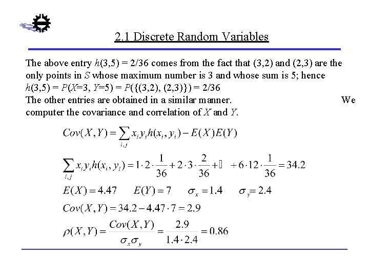
2. 1 Discrete Random Variables The above entry h(3, 5) = 2/36 comes from the fact that (3, 2) and (2, 3) are the only points in S whose maximum number is 3 and whose sum is 5; hence h(3, 5) = P(X=3, Y=5) = P({(3, 2), (2, 3)}) = 2/36 The other entries are obtained in a similar manner. We computer the covariance and correlation of X and Y.

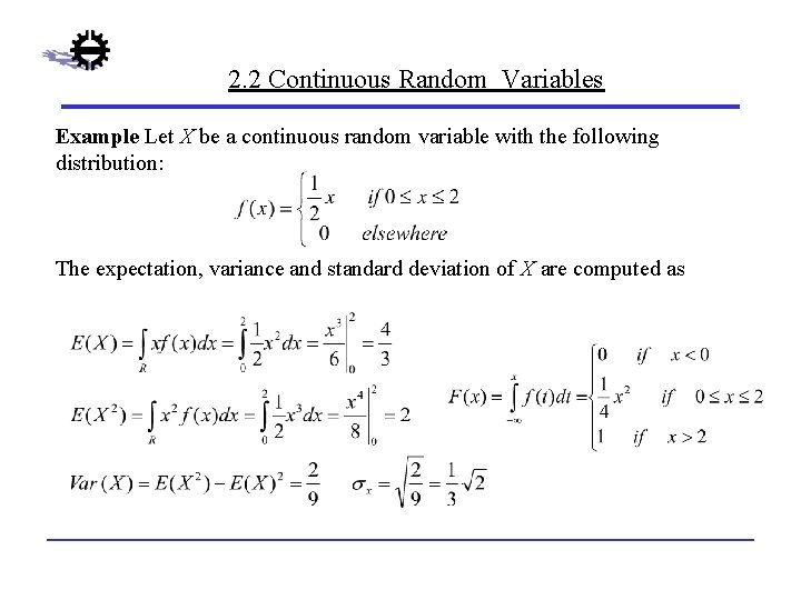
2. 2 Continuous Random Variables Example Let X be a continuous random variable with the following distribution: The expectation, variance and standard deviation of X are computed as

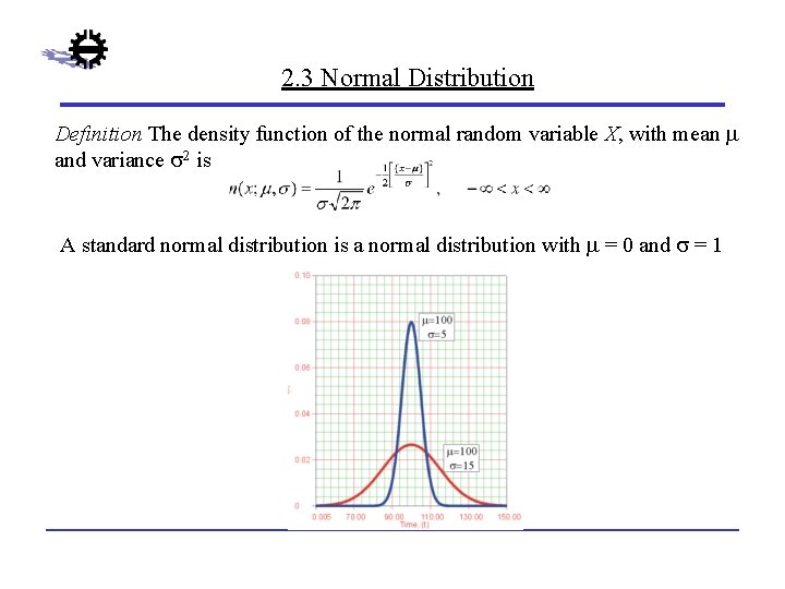
2. 3 Normal Distribution Definition The density function of the normal random variable X, with mean and variance 2 is A standard normal distribution is a normal distribution with = 0 and = 1

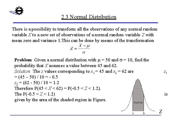
2. 3 Normal Distribution There is a possibility to transform all the observations of any normal random variable X to a new set of observations of a normal random variable Z with mean zero and variance 1. This can be done by means of the transformation Problem Given a normal distribution with = 50 and = 10, find the probability that X assumes a value between 45 and 62. Solution The z values corresponding to x 1 = 45 and x 2 = 62 are = (45 – 50) / 10 = - 0. 5 z 2 = (62 - 50) / 10 = 1. 2 Therefore P(45 < X < 62) = P(-0. 5 < Z < 1. 2). The P(-0. 5 < Z < 1. 2) given by the area of the shaded region in Figure. z 1 is

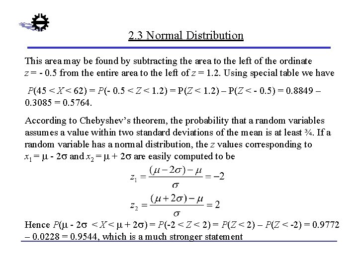
2. 3 Normal Distribution This area may be found by subtracting the area to the left of the ordinate z = - 0. 5 from the entire area to the left of z = 1. 2. Using special table we have P(45 < X < 62) = P(- 0. 5 < Z < 1. 2) = P(Z < 1. 2) – P(Z < - 0. 5) = 0. 8849 – 0. 3085 = 0. 5764. According to Chebyshev’s theorem, the probability that a random variables assumes a value within two standard deviations of the mean is at least ¾. If a random variable has a normal distribution, the z values corresponding to x 1 = - 2 and x 2 = + 2 are easily computed to be Hence P( - 2 < X < + 2 ) = P(-2 < Z < 2) = P(Z < 2) – P(Z < -2) = 0. 9772 – 0. 0228 = 0. 9544, which is a much stronger statement

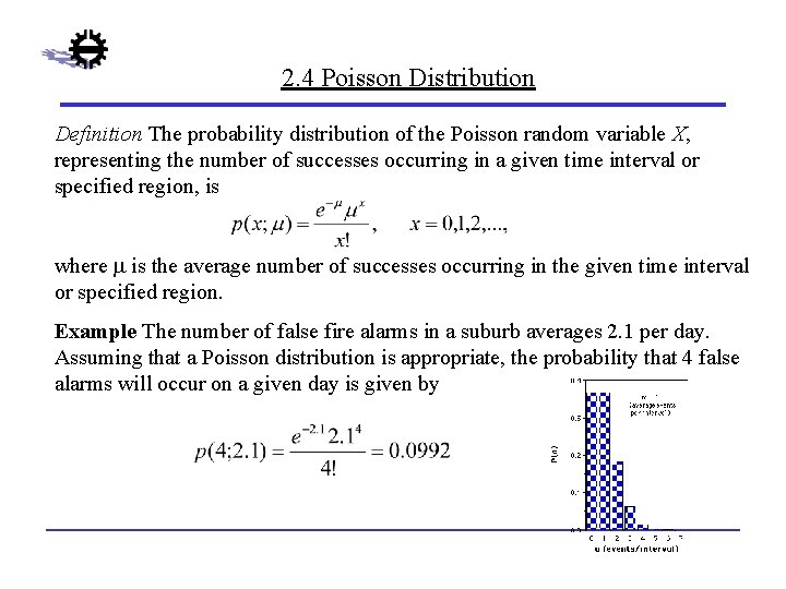
2. 4 Poisson Distribution Definition The probability distribution of the Poisson random variable X, representing the number of successes occurring in a given time interval or specified region, is where is the average number of successes occurring in the given time interval or specified region. Example The number of false fire alarms in a suburb averages 2. 1 per day. Assuming that a Poisson distribution is appropriate, the probability that 4 false alarms will occur on a given day is given by

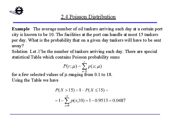
2. 4 Poisson Distribution Example The average number of oil tankers arriving each day at a certain port city is known to be 10. The facilities at the port can handle at most 15 tankers per day. What is the probability that on a given day tankers will have to be sent away? Solution Let X be the number of tankers arriving each day. There are special statistical Table which contains Poisson probability sums for a few selected values of ranging from 0. 1 to 18. Using the Table we have

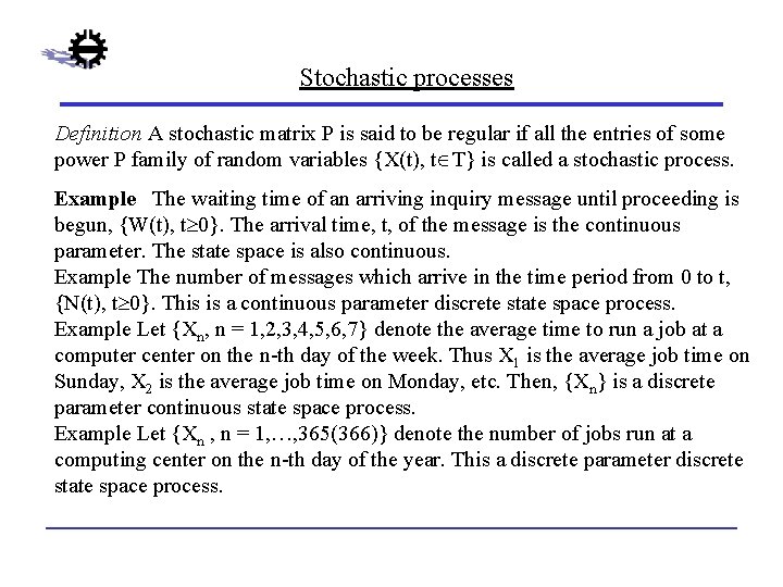
Stochastic processes Definition A stochastic matrix P is said to be regular if all the entries of some power P family of random variables {X(t), t T} is called a stochastic process. Example The waiting time of an arriving inquiry message until proceeding is begun, {W(t), t 0}. The arrival time, t, of the message is the continuous parameter. The state space is also continuous. Example The number of messages which arrive in the time period from 0 to t, {N(t), t 0}. This is a continuous parameter discrete state space process. Example Let {Xn, n = 1, 2, 3, 4, 5, 6, 7} denote the average time to run a job at a computer center on the n-th day of the week. Thus X 1 is the average job time on Sunday, X 2 is the average job time on Monday, etc. Then, {Xn} is a discrete parameter continuous state space process. Example Let {Xn , n = 1, …, 365(366)} denote the number of jobs run at a computing center on the n-th day of the year. This a discrete parameter discrete state space process.

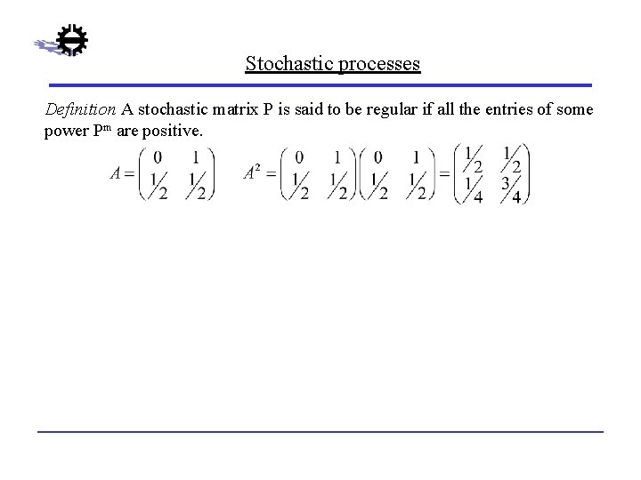
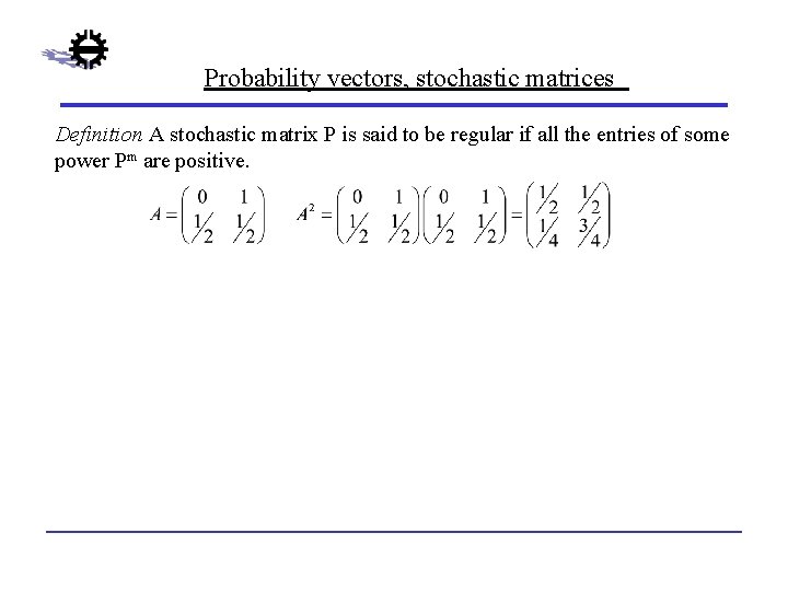
Stochastic processes Definition A stochastic matrix P is said to be regular if all the entries of some power Pm are positive.

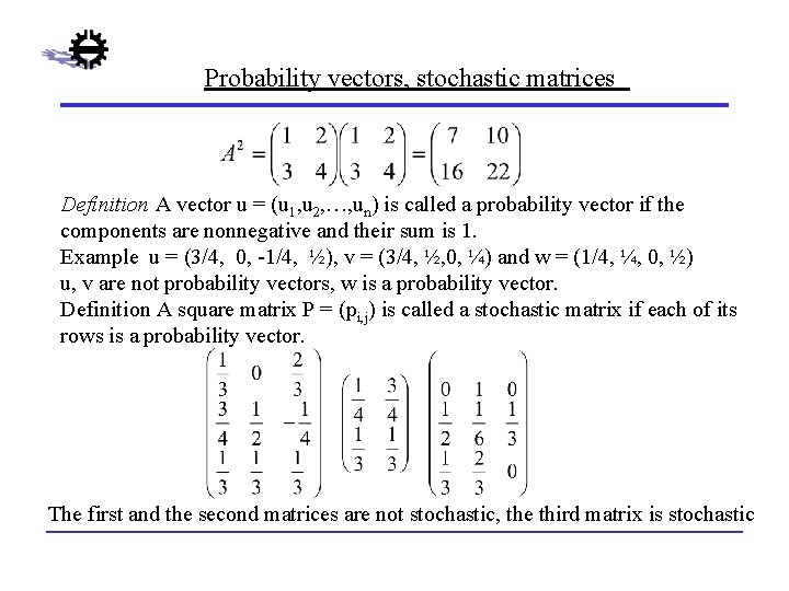
Probability vectors, stochastic matrices Definition A vector u = (u 1, u 2, …, un) is called a probability vector if the components are nonnegative and their sum is 1. Example u = (3/4, 0, -1/4, ½), v = (3/4, ½, 0, ¼) and w = (1/4, ¼, 0, ½) u, v are not probability vectors, w is a probability vector. Definition A square matrix P = (pi, j) is called a stochastic matrix if each of its rows is a probability vector. The first and the second matrices are not stochastic, the third matrix is stochastic

Probability vectors, stochastic matrices Definition A stochastic matrix P is said to be regular if all the entries of some power Pm are positive.