Supply Chain Management Lecture 21 Outline Today Finish

Supply Chain Management Lecture 21

Outline • Today – Finish Chapter 11 • Sections 1, 2, 3, 7, 8 – Skipping 11. 2 “Evaluating Safety Inventory Given Desired Fill rate” – Start with Chapter 12 • Sections 1, 2, 3 – Section 2 up to and including Example 12. 2 • Friday – Homework 5 online • Due Thursday April 8 before class • Next week – Finish Chapter 12 – Start with Chapter 14

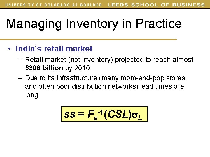
Managing Inventory in Practice • India’s retail market – Retail market (not inventory) projected to reach almost $308 billion by 2010 – Due to its infrastructure (many mom-and-pop stores and often poor distribution networks) lead times are long ss = Fs-1(CSL) L

Managing Inventory in Practice • Department of Defense – DOD reported (1995) that it had a secondary inventory (spare and repair parts, clothing, medical supplies, and other items) to support its operating forces valued at $69. 6 billion – About half of the inventory includes items that are not needed to be on hand to support DOD war reserve or current operating requirements

Safety Inventory A new technology allows books to be printed in ten minutes. Borders has decided to purchase these machines for each store. They must decide which books to carry in stock and which books to print on demand using this technology. Would you recommend Borders to use the new technology for best-sellers or for other books?

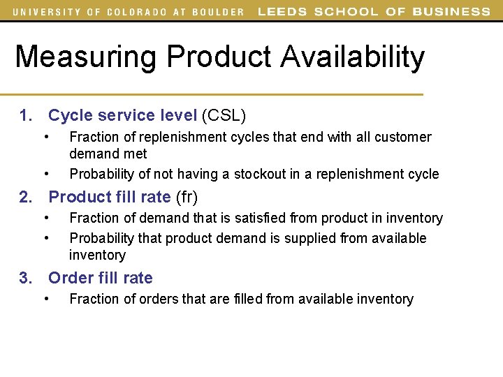
Measuring Product Availability 1. Cycle service level (CSL) • • Fraction of replenishment cycles that end with all customer demand met Probability of not having a stockout in a replenishment cycle 2. Product fill rate (fr) • • Fraction of demand that is satisfied from product in inventory Probability that product demand is supplied from available inventory 3. Order fill rate • Fraction of orders that are filled from available inventory

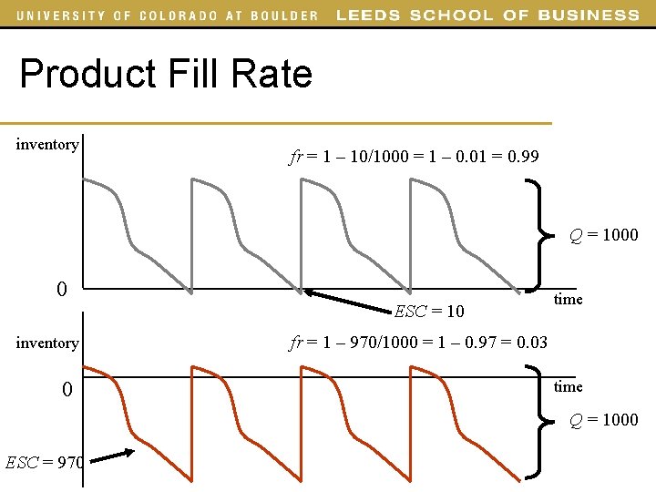
Product Fill Rate inventory fr = 1 – 10/1000 = 1 – 0. 01 = 0. 99 Q = 1000 0 ESC = 10 inventory 0 time fr = 1 – 970/1000 = 1 – 0. 97 = 0. 03 time Q = 1000 ESC = 970

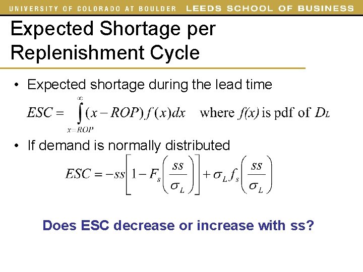
Expected Shortage per Replenishment Cycle • Expected shortage during the lead time • If demand is normally distributed Does ESC decrease or increase with ss?

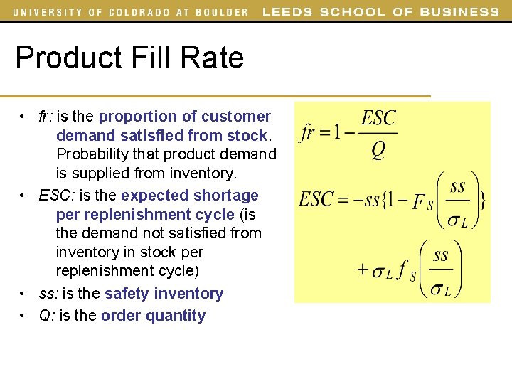
Product Fill Rate • fr: is the proportion of customer demand satisfied from stock. Probability that product demand is supplied from inventory. • ESC: is the expected shortage per replenishment cycle (is the demand not satisfied from inventory in stock per replenishment cycle) • ss: is the safety inventory • Q: is the order quantity

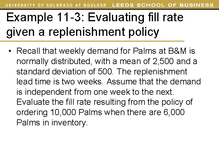
Example 11 -3: Evaluating fill rate given a replenishment policy • Recall that weekly demand for Palms at B&M is normally distributed, with a mean of 2, 500 and a standard deviation of 500. The replenishment lead time is two weeks. Assume that the demand is independent from one week to the next. Evaluate the fill rate resulting from the policy of ordering 10, 000 Palms when there are 6, 000 Palms in inventory.

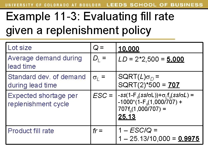
Example 11 -3: Evaluating fill rate given a replenishment policy Lot size Average demand during lead time Q= DL = 10, 000 LD = 2*2, 500 = 5, 000 Standard dev. of demand during lead time Expected shortage per replenishment cycle L = SQRT(L) D = SQRT(2)*500 = 707 ESC = -ss(1 -Fs(ss/ L))+ Lfs(ss/ L) = -1000*(1 -Fs(1, 000/707) + 707 fs(1, 000/707) = 25. 13 Product fill rate fr = 1 – ESC/Q = 1 – 25. 13/10, 000 = 0. 9975

Cycle Service Level versus Fill Rate What happens to CSL and fr when the safety inventory (ss) increases? What happens to CSL and fr when the lot size (Q) increases?

Lead Time Uncertainty Why do some firms have zero tolerance for early/late deliveries?

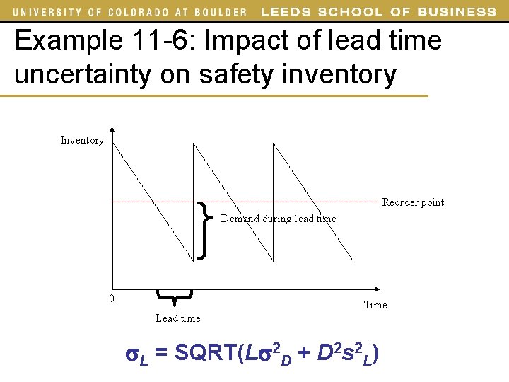
Example 11 -6: Impact of lead time uncertainty on safety inventory Inventory Reorder point Demand during lead time 0 Time Lead time L = SQRT(L 2 D + D 2 s 2 L)

Example 11 -6: Impact of lead time uncertainty on safety inventory • Daily demand at Dell is normally distributed, with a mean of 2, 500 and a standard deviation of 500. A key component in PC assembly is the hard drive. The hard drive supplier takes an average of L = 7 days to replenish inventory at Dell is targeting a CSL of 90 percent for its hard drive inventory. Evaluate the safety inventory of hard drives that Dell must carry if the standard deviation of the lead time is 7 days.

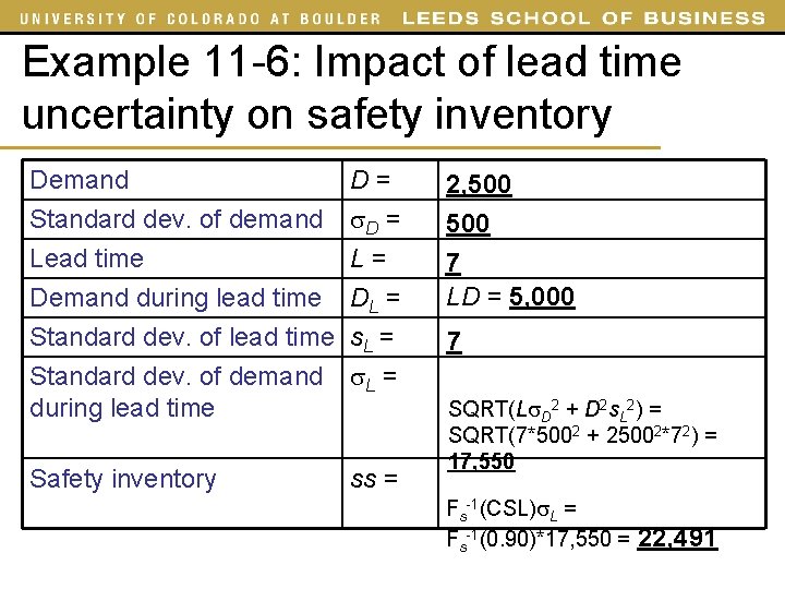
Example 11 -6: Impact of lead time uncertainty on safety inventory Demand Standard dev. of demand Lead time Demand during lead time Standard dev. of demand during lead time D= D = L= DL = s. L = Safety inventory ss = 2, 500 7 LD = 5, 000 7 SQRT(L D 2 + D 2 s. L 2) = SQRT(7*5002 + 25002*72) = 17, 550 Fs-1(CSL) L = Fs-1(0. 90)*17, 550 = 22, 491

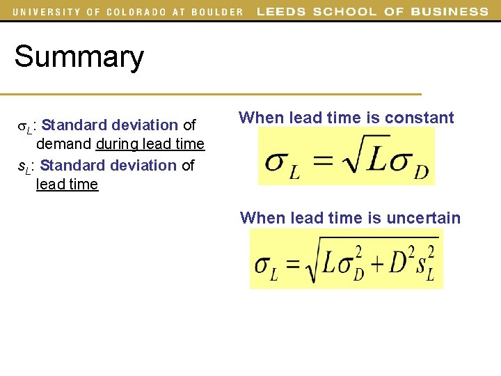
Summary L: Standard deviation of demand during lead time s. L: Standard deviation of lead time When lead time is constant When lead time is uncertain

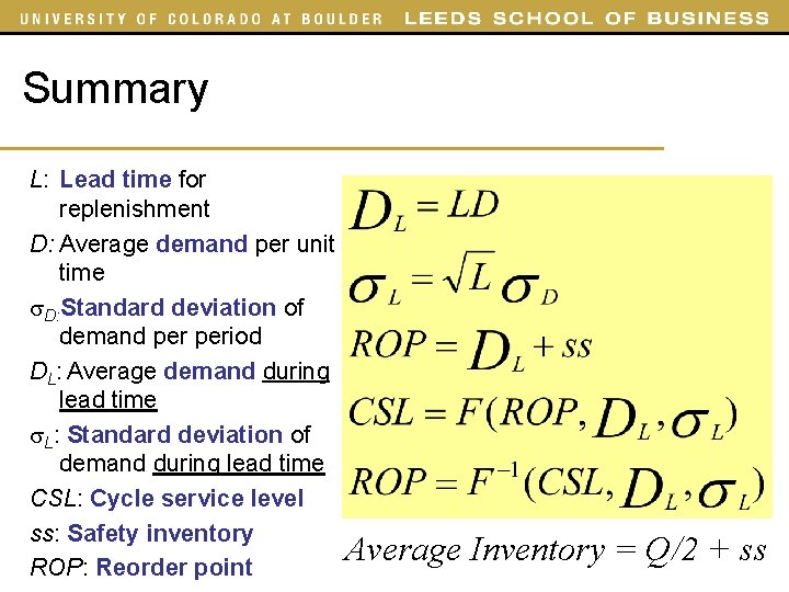
Summary L: Lead time for replenishment D: Average demand per unit time D: Standard deviation of demand period DL: Average demand during lead time L: Standard deviation of demand during lead time CSL: Cycle service level ss: Safety inventory ROP: Reorder point Average Inventory = Q/2 + ss

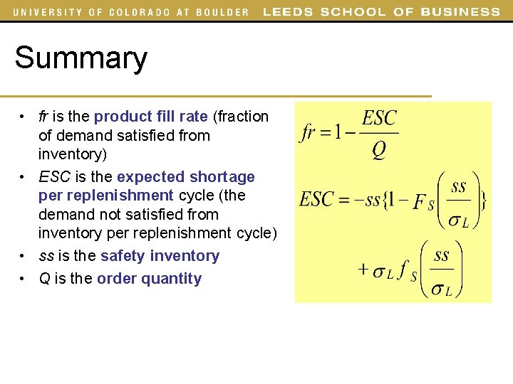
Summary • fr is the product fill rate (fraction of demand satisfied from inventory) • ESC is the expected shortage per replenishment cycle (the demand not satisfied from inventory per replenishment cycle) • ss is the safety inventory • Q is the order quantity

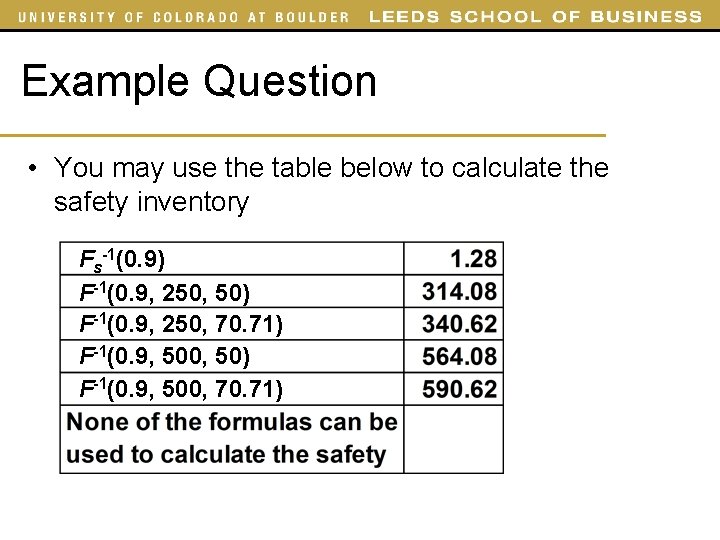
Example Question • Weekly demand for canned fruit at a grocery store is normally distributed, with a mean of 250 and a standard deviation of 50. The lead time is two weeks. Assuming a continuous review replenishment policy, how much safety inventory should the store carry to achieve a CSL of 90 percent?

Example Question • You may use the table below to calculate the safety inventory Fs-1(0. 9) F-1(0. 9, 250, 50) F-1(0. 9, 250, 70. 71) F-1(0. 9, 500, 50) F-1(0. 9, 500, 70. 71)

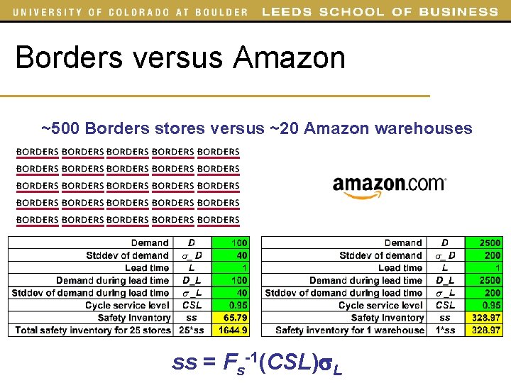
Safety Inventory Why is Amazon. com able to provide a large variety of books and music with less safety inventory than a bookstore chain selling through retail stores?

Borders versus Amazon ~500 Borders stores versus ~20 Amazon warehouses ss = Fs-1(CSL) L

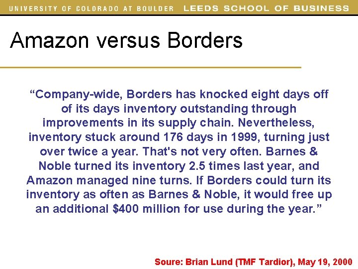
Amazon versus Borders “Company-wide, Borders has knocked eight days off of its days inventory outstanding through improvements in its supply chain. Nevertheless, inventory stuck around 176 days in 1999, turning just over twice a year. That's not very often. Barnes & Noble turned its inventory 2. 5 times last year, and Amazon managed nine turns. If Borders could turn its inventory as often as Barnes & Noble, it would free up an additional $400 million for use during the year. ” Soure: Brian Lund (TMF Tardior), May 19, 2000

Safety Inventory In the 1980 s, paint was sold by color and size in paint retail stores. Today paint is mixed at the paint store according to the color desired. What impact did this change had on safety inventories in the supply chain?

Importance of the Level of Product Availability • Product availability (also known as customer service level) is measured by – CSL (Cycle service level) – fr (Product fill rate) • Product availability affects supply chain responsiveness and costs – High levels of product availability increased responsiveness and higher revenues – High levels of product availability increased inventory levels and higher costs

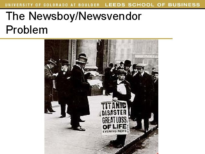
The Newsboy/Newsvendor Problem

The Newsboy/Newsvendor Problem • One time decision under uncertainty – Demand is uncertain – Plan inventory for a single cycle • Trade-off – Ordering too much • (waste, salvage value < cost) – Ordering too little • (excess demand is lost) • Examples – Restaurants – Fashion – High tech

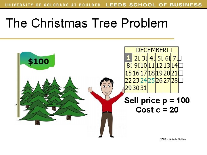
The Christmas Tree Problem Sell price p = 100 Cost c = 20

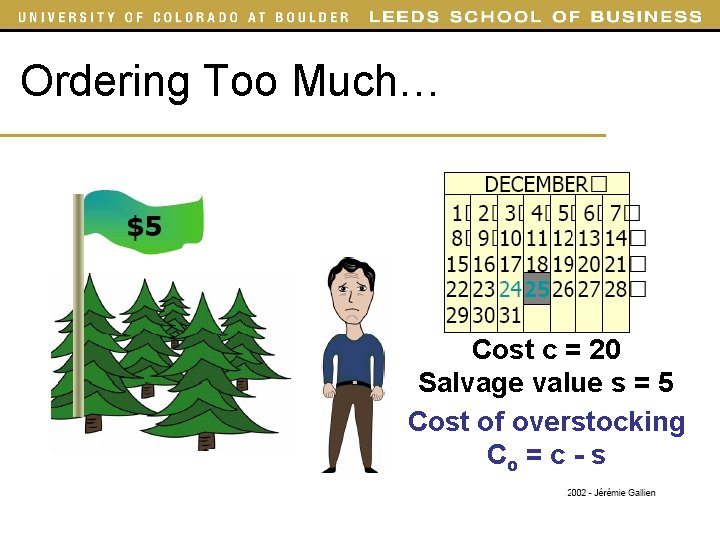
Ordering Too Much… Cost c = 20 Salvage value s = 5 Cost of overstocking Co = c - s

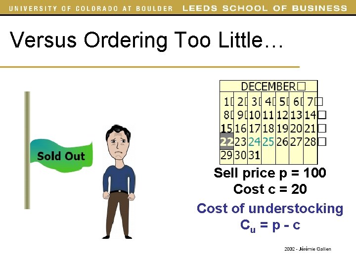
Versus Ordering Too Little… Sell price p = 100 Cost c = 20 Cost of understocking Cu = p - c

Factors Affecting the Optimal Level of Product Availability • Cost of overstocking (Co = c – s) – The loss incurred by a firm for each unsold unit at the end of the selling season • Cost of understocking (Cu = p – c) – The margin lost by a firm for each lost sale because there is no inventory on hand • Includes the margin lost from current as well as future sales if the customer does not return

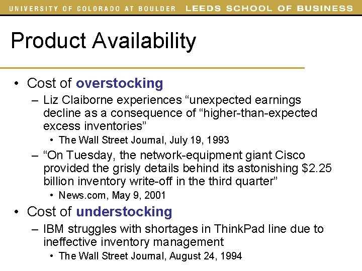
Product Availability • Cost of overstocking – Liz Claiborne experiences “unexpected earnings decline as a consequence of “higher-than-expected excess inventories” • The Wall Street Journal, July 19, 1993 – “On Tuesday, the network-equipment giant Cisco provided the grisly details behind its astonishing $2. 25 billion inventory write-off in the third quarter” • News. com, May 9, 2001 • Cost of understocking – IBM struggles with shortages in Think. Pad line due to ineffective inventory management • The Wall Street Journal, August 24, 1994

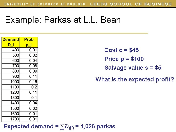
Example: Parkas at L. L. Bean Cost c = $45 Price p = $100 Salvage value s = $5 What is the expected profit? Expected demand = ∑Dipi = 1, 026 parkas

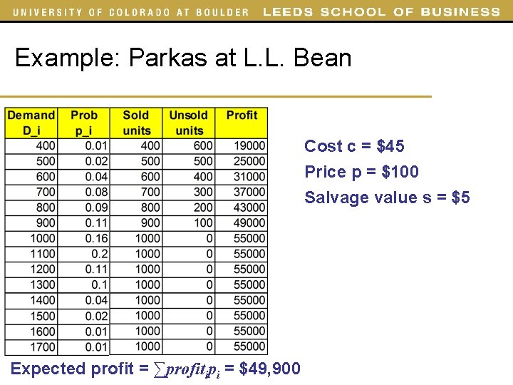
Example: Parkas at L. L. Bean Cost c = $45 Price p = $100 Salvage value s = $5 Expected profit = ∑profitipi = $49, 900

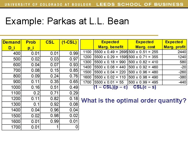
Example: Parkas at L. L. Bean (1 – CSL)(p – c) CSL(c – s) What is the optimal order quantity?

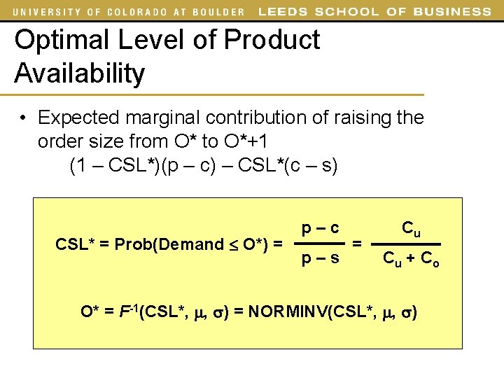
Optimal Level of Product Availability • Expected marginal contribution of raising the order size from O* to O*+1 (1 – CSL*)(p – c) – CSL*(c – s) p – c CSL* = Prob(Demand O*) = = p – s Cu Cu + Co O* = F-1(CSL*, , ) = NORMINV(CSL*, , )

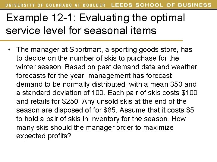
Example 12 -1: Evaluating the optimal service level for seasonal items • The manager at Sportmart, a sporting goods store, has to decide on the number of skis to purchase for the winter season. Based on past demand data and weather forecasts for the year, management has forecast demand to be normally distributed, with a mean 350 and a standard deviation of 100. Each pair of skis costs $100 and retails for $250. Any unsold skis at the end of the season are disposed of for $85. Assume that it costs $5 to hold a pair of skis in inventory for the season. How many skis should the manager order to maximize expected profits?

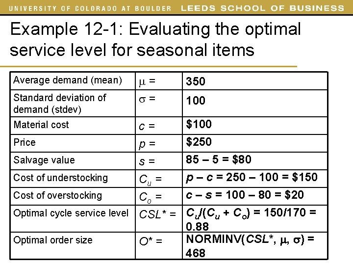
Example 12 -1: Evaluating the optimal service level for seasonal items Average demand (mean) Standard deviation of demand (stdev) Material cost = = 350 c= $100 Price p= Salvage value s= Cost of understocking Cu = Cost of overstocking Co = Optimal cycle service level CSL* = Optimal order size O* = 100 $250 85 – 5 = $80 p – c = 250 – 100 = $150 c – s = 100 – 80 = $20 Cu/(Cu + Co) = 150/170 = 0. 88 NORMINV(CSL*, , ) = 468