Matching Supply with Demand An Introduction to Operations

Matching Supply with Demand: An Introduction to Operations Management Gérard Cachon Christian. Terwiesch All slides in this file are copyrighted by Gerard Cachon and Christian Terwiesch. Any instructor that adopts Matching Supply with Demand: An Introduction to Operations Management as a required text for their course is free to use and modify these slides as desired. All others must obtain explicit written permission from the authors to use these slides. Slide 1

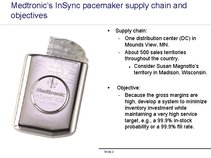
Medtronic’s In. Sync pacemaker supply chain and objectives § Supply chain: - One distribution center (DC) in Mounds View, MN. - About 500 sales territories throughout the country. Consider Susan Magnotto’s territory in Madison, Wisconsin. u § Slide 2 Objective: - Because the gross margins are high, develop a system to minimize inventory investment while maintaining a very high service target, e. g. , a 99. 9% in-stock probability or a 99. 9% fill rate.

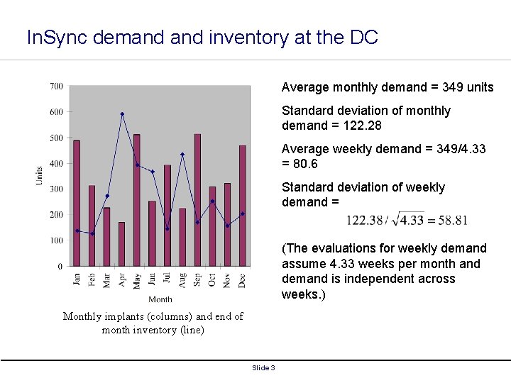
In. Sync demand inventory at the DC Average monthly demand = 349 units Standard deviation of monthly demand = 122. 28 Average weekly demand = 349/4. 33 = 80. 6 Standard deviation of weekly demand = (The evaluations for weekly demand assume 4. 33 weeks per month and demand is independent across weeks. ) Monthly implants (columns) and end of month inventory (line) Slide 3

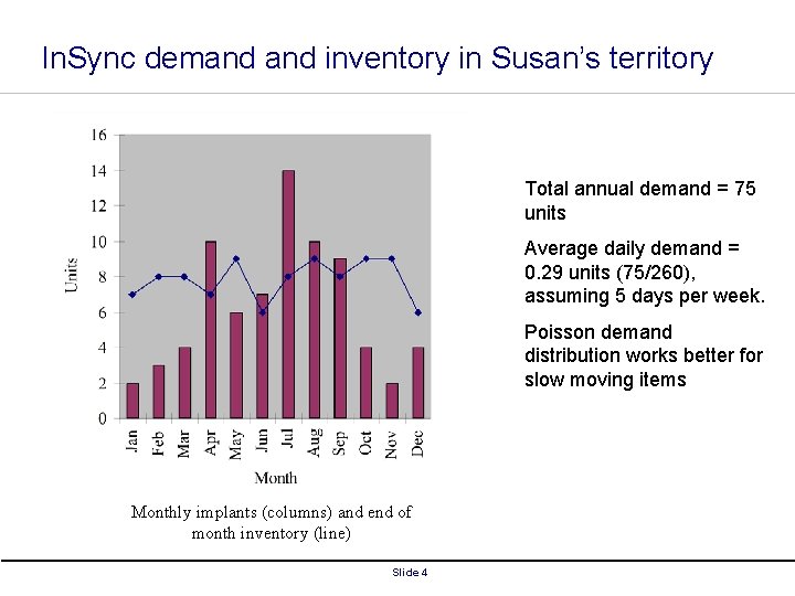
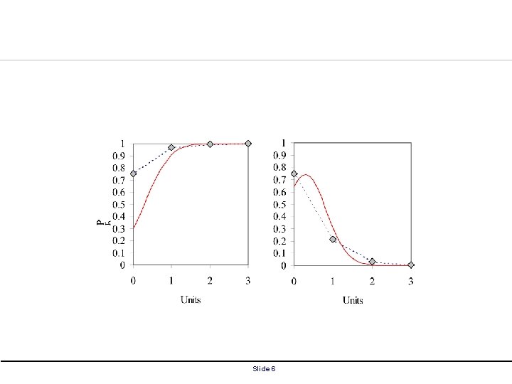
In. Sync demand inventory in Susan’s territory Total annual demand = 75 units Average daily demand = 0. 29 units (75/260), assuming 5 days per week. Poisson demand distribution works better for slow moving items Monthly implants (columns) and end of month inventory (line) Slide 4

Slide 5

Slide 6

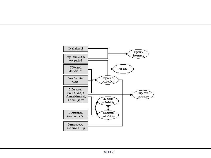
Lead time, l Pipeline inventory Exp. demand in one period If Normal demand, s Loss function table Order up-to level, S, and, if Normal demand, z = (S – m) /s Distribution function table Fill rate Expected backorder In-stock probability Stockout probability Demand over lead time + 1, m Slide 7 Expected inventory

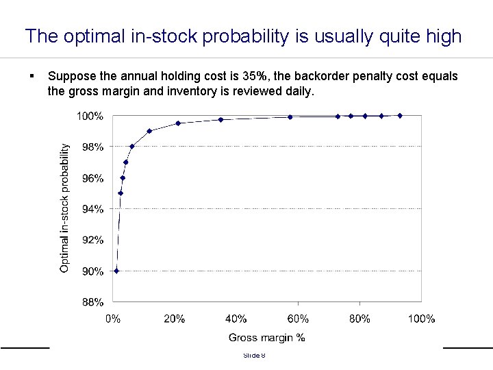
The optimal in-stock probability is usually quite high § Suppose the annual holding cost is 35%, the backorder penalty cost equals the gross margin and inventory is reviewed daily. Slide 8

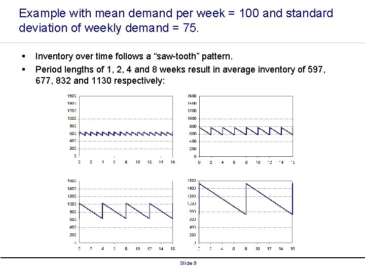
Example with mean demand per week = 100 and standard deviation of weekly demand = 75. § § Inventory over time follows a “saw-tooth” pattern. Period lengths of 1, 2, 4 and 8 weeks result in average inventory of 597, 677, 832 and 1130 respectively: Slide 9

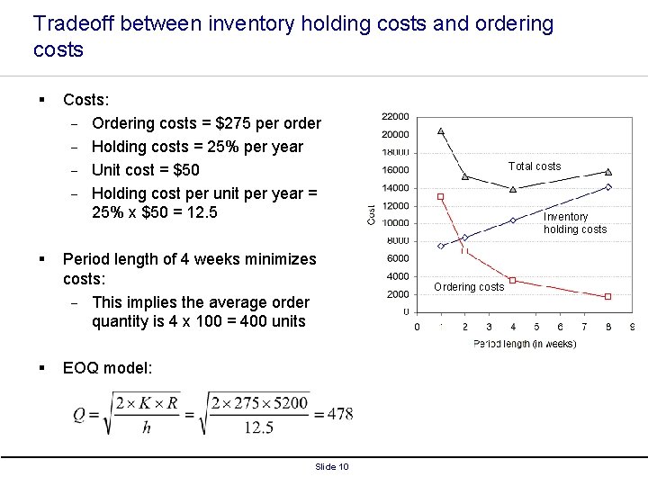
Tradeoff between inventory holding costs and ordering costs § § § Costs: - Ordering costs = $275 per order - Holding costs = 25% per year - Unit cost = $50 - Holding cost per unit per year = 25% x $50 = 12. 5 Period length of 4 weeks minimizes costs: - This implies the average order quantity is 4 x 100 = 400 units EOQ model: Slide 10 Total costs Inventory holding costs Ordering costs

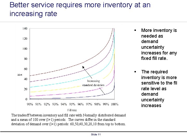
Better service requires more inventory at an increasing rate The tradeoff between inventory and fill rate with Normally distributed demand a mean of 100 over (l+1) periods. The curves differ in the standard deviation of demand over (l+1) periods: 60, 50, 40, 30, 20, 10 from top to bottom. Slide 11 § More inventory is needed as demand uncertainty increases for any fixed fill rate. § The required inventory is more sensitive to the fil rate level as demand uncertainty increases

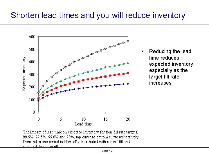
Shorten lead times and you will reduce inventory § The impact of lead time on expected inventory for four fill rate targets, 99. 9%, 99. 5%, 99. 0% and 98%, top curve to bottom curve respectively. Demand in one period is Normally distributed with mean 100 and standard deviation 60. Slide 12 Reducing the lead time reduces expected inventory, especially as the target fill rate increases

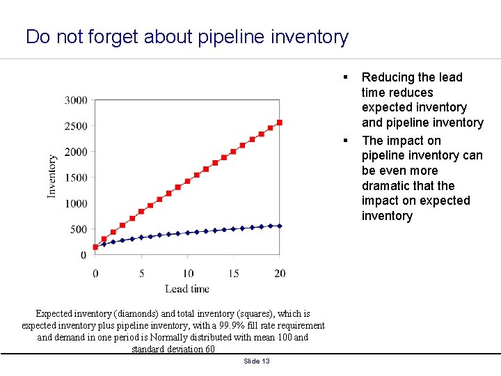
Do not forget about pipeline inventory § § Expected inventory (diamonds) and total inventory (squares), which is expected inventory plus pipeline inventory, with a 99. 9% fill rate requirement and demand in one period is Normally distributed with mean 100 and standard deviation 60 Slide 13 Reducing the lead time reduces expected inventory and pipeline inventory The impact on pipeline inventory can be even more dramatic that the impact on expected inventory

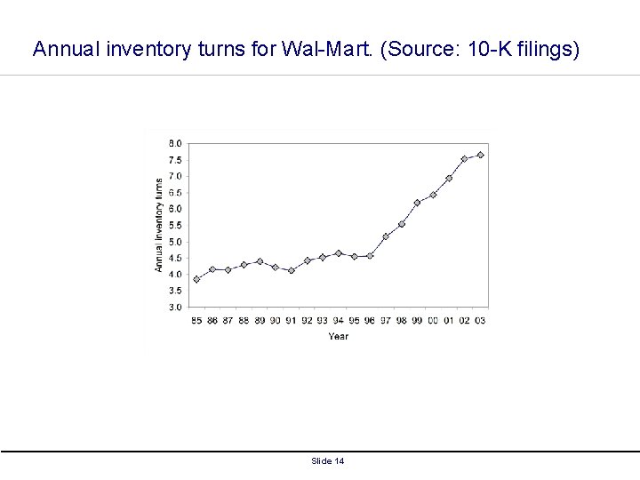
Annual inventory turns for Wal-Mart. (Source: 10 -K filings) Slide 14