Supply Chain Management Supply Chain Management First appearance

Supply Chain Management

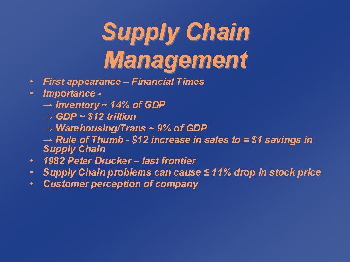
Supply Chain Management • First appearance – Financial Times • Importance → Inventory ~ 14% of GDP → GDP ~ $12 trillion → Warehousing/Trans ~ 9% of GDP → Rule of Thumb - $12 increase in sales to = $1 savings in Supply Chain • 1982 Peter Drucker – last frontier • Supply Chain problems can cause ≤ 11% drop in stock price • Customer perception of company

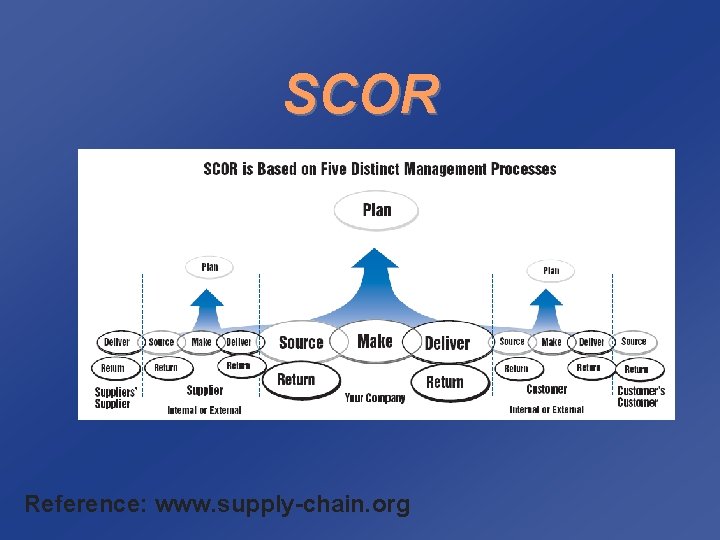
SCOR Reference: www. supply-chain. org

Supply Chain ü All activities associated with the flow and transformation of goods and services from raw materials to the end user, the customer ü A sequence of business activities from suppliers through customers that provide the products, services, and information to achieve customer satisfaction

Supply Chain “The global network used to deliver products and services from raw materials to end customers through an engineered flow of information, physical distribution, and cash. ” APICS Dictionary, 10 th ed.

Supply Chain Management ü Synchronization of activities required to achieve maximum competitive benefits ü Coordination, cooperation, and communication ü Rapid flow of information ü Vertical integration

Supply Chain Uncertainty ü Forecasting, lead times, batch ordering, price fluctuations, and inflated orders contribute to variability ü Inventory is a form of insurance ü Distorted information is one of the main causes of uncertainty Bullwhip effect

Information in the Supply Chain ü Centralized coordination of information flows ü Integration of transportation, distribution, ordering, and production ü Direct access to domestic and global transportation and distribution channels ü Locating and tracking the movement of every item in the supply chain - RFID

Information in the Supply Chain ü Consolidation of purchasing from all suppliers ü Intercompany and intracompany information access ü Electronic Data Interchange ü Data acquisition at the point of origin and point of sale ü Instantaneous updating of inventory levels ü Visibility

Electronic Business In Theory: ü Replacement of physical processes with electronic ones ü Cost and price reductions ü Reduction or elimination of intermediaries ü Shortening transaction times for ordering and delivery ü Wider presence and increased visibility

Electronic Business ü Greater choices and more information for customers ü Improved service ü Collection and analysis of customer data and preferences ü Virtual companies with lower prices ü Leveling the playing field for smaller companies ü Gain global access to markets & customers

Electronic Data Interchange ü Computer-to-computer exchange of business documents in a standard format ü Quick access, better customer service, less paperwork, better communication, increased productivity, improved tracing and expediting, improves billing and cost efficiency

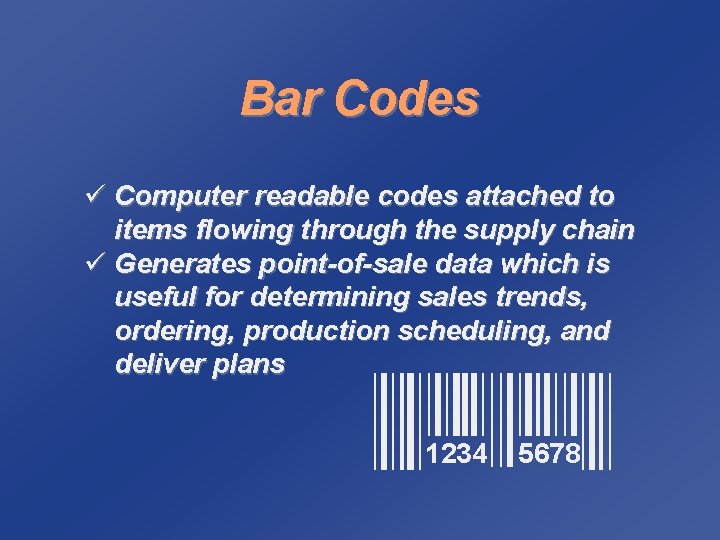
Bar Codes ü Computer readable codes attached to items flowing through the supply chain ü Generates point-of-sale data which is useful for determining sales trends, ordering, production scheduling, and deliver plans 1234 5678

IT Issues ü Increased benefits and sophistication come with increased costs ü Efficient web sites do not necessarily mean the rest of the supply chain will be as efficient ü Security problems are very real – camera phones, cell phones, thumb drives ü Collaboration and trust are important elements that may be new to business relationships

Suppliers ü Purchased materials account for about half of manufacturing costs ü Materials, parts, and service must be delivered on time, of high quality, and low cost ü Suppliers should be integrated into their customers’ supply chains ü Partnerships should be established ü On-demand delivery (JIT) is a frequent requirement - what is JIT and does it work?

Sourcing ü Relationship between customers and suppliers focuses on collaboration and cooperation ü Outsourcing has become a long-term strategic decision ü Organizations focus on core competencies How does ü Single-sourcing is single source increasingly a part differ from sole of supplier relations source?

Distribution ü The actual movement of products and materials between locations ü Handling of materials and products at receiving docks, storing products, packaging, and shipping ü Often called logistics ü Driving force today is speed ü Particularly important for Internet dot-coms

Distribution Centers and Warehousing ü DCs are some of the largest business facilities in the United States ü Trend is for more frequent orders in smaller quantities ü Flow-through facilities and automated material handling ü Final assembly and product configuration (postponement) may be done at the DC

Warehouse Management Systems ü Highly automated systems ü A good system will control item slotting, pick lists, packing, and shipping ü Most newer systems include transportation management (load management/configuration), order management, yard management, labor management, warehouse optimization

Vendor-Managed Inventory ü Not a new concept – same process used by bread deliveries to stores for decades ü Reduces need for warehousing ü Increased speed, reduced errors, and improved service ü Onus is on the supplier to keep the shelves full or assembly lines running ü variation of JIT ü Proctor&Gamble - Wal-Mart ü DLA – moving from a manager of supplies to a manager of suppliers ü Direct Vendor Deliveries – loss of visibility

Collaborative Distribution and Outsourcing ü Collaborative planning, forecasting, and replenishment (CPFR) started by Nabisco ü Allows suppliers to know what is really needed and when ü Electronic-based exchange of data and information ü Significant decrease in inventory levels and more efficient logistics - maybe not! ü Companies work together for benefit of all of the supply chain

Transportation ü Common methods are railroads, trucking, water, air, intermodal, package carriers, and pipelines

Railroads ü 150, 000 miles in US ü Low cost, high-volume ü Improving flexibility ü intermodal service ü double stacking Complaints: slow, inflexible, large loads Advantages: large/bulky loads, intermodal

Award-Winning Service Recognition Wal-Mart Stores, Inc. Carrier of the Year – 5 years in a row Target Only rail carrier to receive the Vice President’s Award Federal Express United Parcel Service 99. 5% failure free, damage free and on-time rating from United Parcel Service every year since 1995 American Honda Motor Company Premier Partner – 4 consecutive years Only rail carrier to receive outstanding supplier award - 2 years in a row Toyota’s North American Parts and Logistics Division (NAPLD) Rail Carrier of the Year – 3 consecutive years Schneider KIA Carrier of the Year – 3 consecutive years Carrier of the Year

Trucking ü Most used mode in US -75% of total freight (not total weight) ü Flexible, small loads ü Consolidation, Internet load match sites ü Single sourcing reduces number of trucking firms serving a company ü Truck load (TL) vs. Less Than Truck Load (LTL)

Air ü Rapidly growing segment of transportation industry ü Lightweight, small items ü Quick, reliable, expensive (relatively expensive depending on costs of not getting item there) ü Major airlines and US Postal Service, UPS, Fed. Ex, DHL

Package Carriers ü Fed. Ex, UPS, US Postal Service, DHL ü Significant growth driven by e-businesses and the move to smaller shipments and consumer desire to have it NOW ü Use several modes of transportation ü Expensive - relative!! ü Fast and reliable - relative!! ü Innovative use of technologies in some cases ü Online tracking – some better than others

Intermodal ü Combination of several modes of transportation ü Most common are truck/rail/truck and truck/water/rail/truck ü Enabled by the use of containers – the development of the 20 and 40 foot containers significantly changed the face of shipping ü ~2% of all US cargo via intermodal

Water ü One of oldest means of transport ü Low-cost, high-volume, slow (relative) ü Security - sheer volume - millions of containers annually ü Bulky, heavy and/or large items ü Standardized shipping containers improve service ü The most common form of international shipping

Pipelines ü Primarily for oil & refined oil products ü Slurry lines carry coal or kaolin ü High initial capital investment ü Low operating costs ü Can cross difficult terrain

Global Supply Chain ü Free trade & global opportunities ü Nations form trading groups ü No tariffs or duties ü Freely transport goods across borders ü Security!!

Global Supply Chain Problems ü National and regional differences ü Customs, business practices, and regulations ü Foreign markets are not homogeneous ü Quality can be a major issue

Security • ~ 10+ million containers annually • Customs-Trade Partnership Against Terrorism (CTPAT) • Port Security – SAFE Ports Act; Scanning of all Containers • Cost - $2 billion closing of major port • 66% of all goods into US comes through 20 major ports • 44% through LA/Long Beach • Cost of attack on major port estimated at $20 Billion

Chapter 11 Forecasting

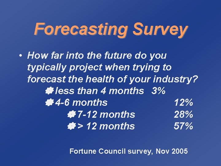
Forecasting Survey • How far into the future do you typically project when trying to forecast the health of your industry? less than 4 months 3% 4 -6 months 12% 7 -12 months 28% > 12 months 57% Fortune Council survey, Nov 2005

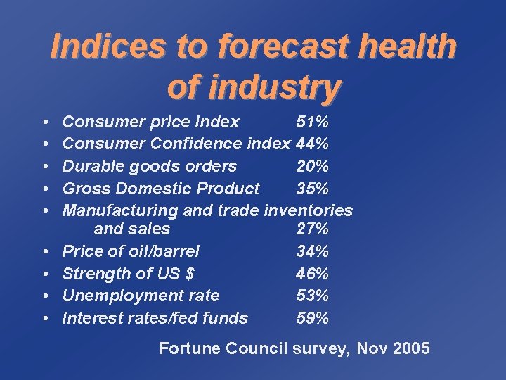
Indices to forecast health of industry • • • Consumer price index 51% Consumer Confidence index 44% Durable goods orders 20% Gross Domestic Product 35% Manufacturing and trade inventories and sales 27% Price of oil/barrel 34% Strength of US $ 46% Unemployment rate 53% Interest rates/fed funds 59% Fortune Council survey, Nov 2005

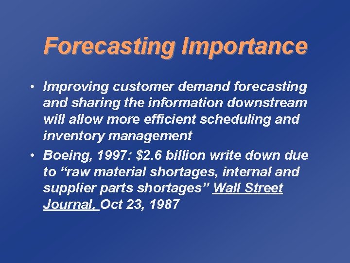
Forecasting Importance • Improving customer demand forecasting and sharing the information downstream will allow more efficient scheduling and inventory management • Boeing, 1997: $2. 6 billion write down due to “raw material shortages, internal and supplier parts shortages” Wall Street Journal, Oct 23, 1987

Forecasting Importance • “Second Quarter sales at US Surgical Corporation decline 25%, resulting in a $22 mil loss…attributed to larger than anticipated inventories on shelves of hospitals. ” US Surgical Quarterly, Jul 1993 • “IBM sells out new Aetna PC; shortage may cost millions in potential revenue. ” Wall Street Journal, Oct 7, 1994

Principles of Forecasting • Forecasts are usually wrong • every forecast should include an estimate of error • Forecasts are more accurate for families or groups • Forecasts are more accurate for nearer periods.

Important Factors to Improve Forecasting • Record Data in the same terms as needed in the forecast – production data for production forecasts; time periods • Record circumstances related to the data • Record the demand separately for different customer groups

Forecast Techniques • Extrinsic Techniques – projections based on indicators that relate to products – examples • Intrinsic – historical data used to forecast (most common)

Forecasting • Forecasting errors can increase the total cost of ownership for a product - inventory carrying costs - obsolete inventory - lack of sufficient inventory - quality of products due to accepting marginal products to prevent stockout

Forecasting • Essential for smooth operations of business organizations • Estimates of the occurrence, timing, or magnitude of uncertain future events • Costs of forecasting: excess labor; excess materials; expediting costs; lost revenues

Forecasting ü Predicting future events ü Usually demand behavior over a time frame ü Qualitative methods ü Based on subjective methods ü Quantitative methods ü Based on mathematical formulas

Impact of Just-in-Time on Forecasting • Just in time as a inventory method • Just in time as a Continuous process improvement program • Just in time - one on the shelf • Usage factors • Single order vs. Case order

Strategic Role of Forecasting ü Focus on supply chain management ü Short term role of product demand ü Long term role of new products, processes, and technologies ü Focus on Total Quality Management ü Satisfy customer demand ü Uninterrupted product flow with no defective items ü Necessary for strategic planning

Strategic Role of Forecasting ü Focus on supply chain management ü Short term role of product demand ü Long term role of new products, processes, and technologies ü Focus on Total Quality Management ü Satisfy customer demand ü Uninterrupted product flow with no defective items ü Necessary for strategic planning

Total Quality Management • Management approach to long term success through customer satisfaction • Total Quality Control - process of creating and producing quality goods and services that meet the expectations of the customer • quality - conformance to requirements or fitness for use

Trumpet of Doom • As forecast horizon increases, so does the forecasting error (i. e. , accuracy decreases) – shorten horizon by shortening of cycles or flow times • Law of Large Numbers – as volume increases, relative variability decreases – forecasting error is smaller: goal – forecast at aggregate levels; collaborate; standardize parts • Volume and activity increase at end of reporting periods – Krispy Kreme

Components of Forecasting Demand ü Time Frame ü Short-range, mediumrange, long-range ü Demand Behavior ü Trends, cycles, seasonal patterns, random

Time Frame ü Short-range to medium-range ü Daily, weekly monthly forecasts of sales data ü Up to 2 years into the future ü Long-range ü Strategic planning of goals, products, markets ü Planning beyond 2 years into the future

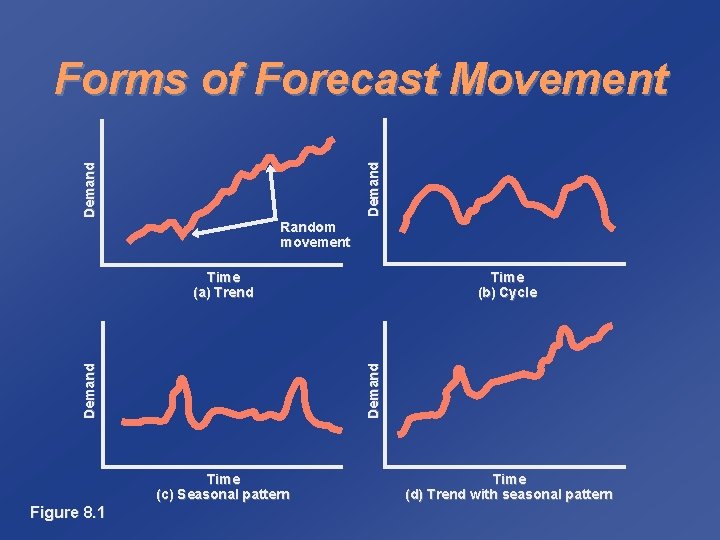
Demand Behavior ü Trend ü gradual, long-term up or down movement ü Cycle ü up & down movement repeating over long time frame ü Seasonal pattern ü periodic oscillation in demand which repeats ü Random movements follow no pattern

Demand Forms of Forecast Movement Random movement Demand Time (c) Seasonal pattern Figure 8. 1 Time (b) Cycle Demand Time (a) Trend Time (d) Trend with seasonal pattern

Forecasting Methods ü Time series ü Regression or causal modeling ü Qualitative methods ü Management judgment, expertise, opinion ü Use management, marketing, purchasing, engineering ü Delphi method ü Solicit forecasts from experts

Time Series Methods ü Statistical methods using historical data ü Moving average ü Exponential smoothing ü Linear trend line ü Assume patterns will repeat ü Naive forecasts ü Forecast = data from last period

Moving Average ü Average several periods of data ü Dampen, smooth out changes ü Use when demand is stable with no trend or seasonal pattern ü stock market analysis - trend analysis

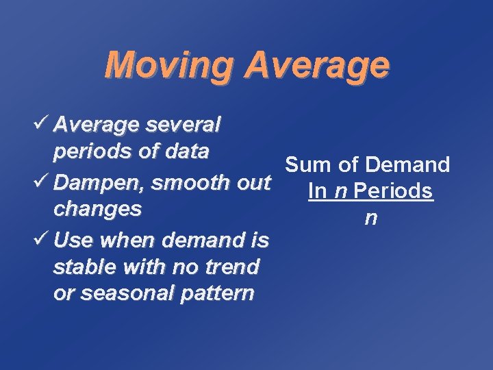
Moving Average ü Average several periods of data Sum of Demand ü Dampen, smooth out In n Periods changes n ü Use when demand is stable with no trend or seasonal pattern

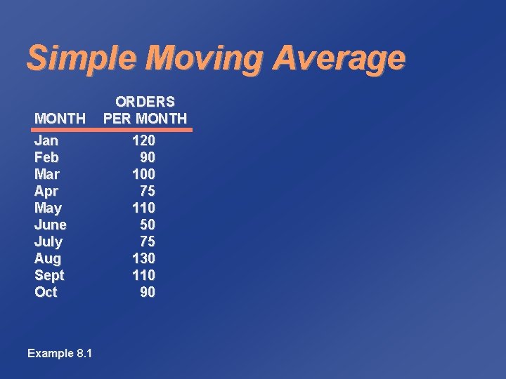
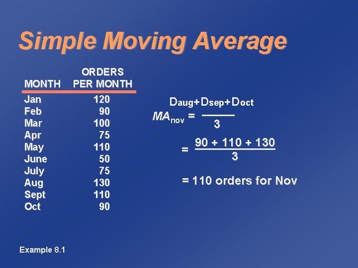
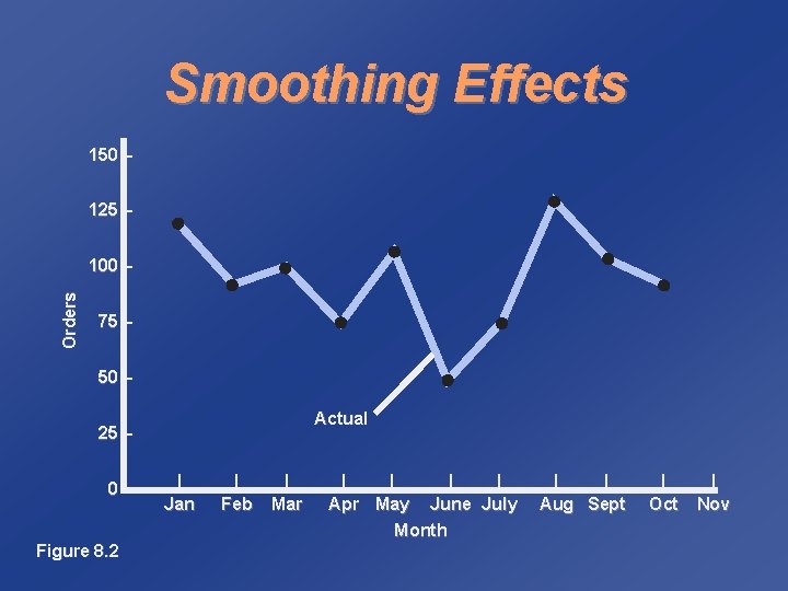
Simple Moving Average MONTH Jan Feb Mar Apr May June July Aug Sept Oct Example 8. 1 ORDERS PER MONTH 120 90 100 75 110 50 75 130 110 90

Simple Moving Average MONTH Jan Feb Mar Apr May June July Aug Sept Oct Example 8. 1 ORDERS PER MONTH 120 90 100 75 110 50 75 130 110 90 Daug+Dsep+Doct MAnov = 3 90 + 110 + 130 = 3 = 110 orders for Nov

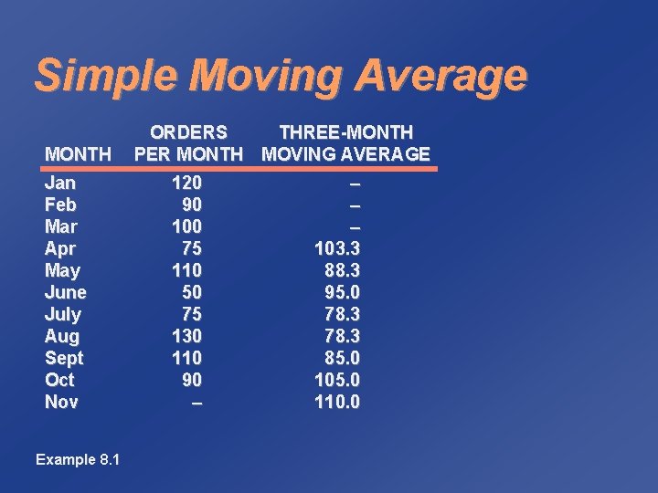
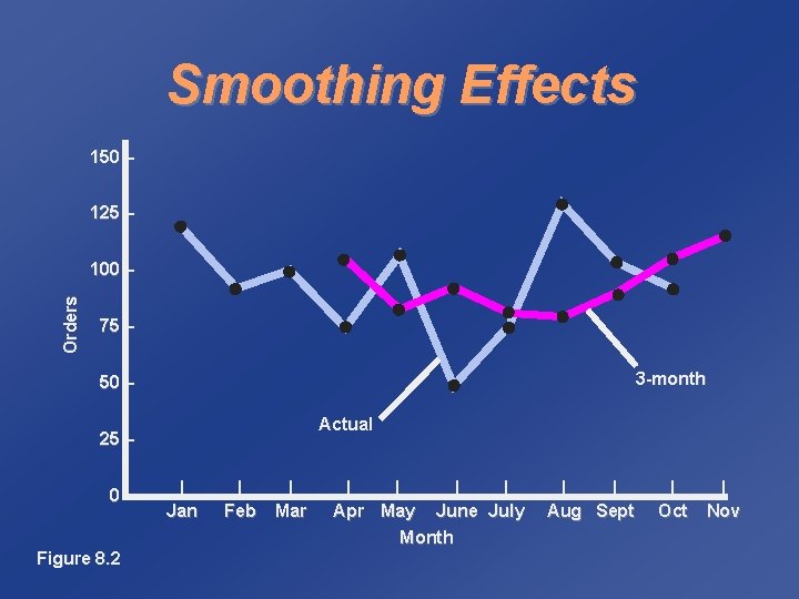
Simple Moving Average MONTH Jan Feb Mar Apr May June July Aug Sept Oct Nov Example 8. 1 ORDERS THREE-MONTH PER MONTH MOVING AVERAGE 120 90 100 75 110 50 75 130 110 90 – – 103. 3 88. 3 95. 0 78. 3 85. 0 105. 0 110. 0

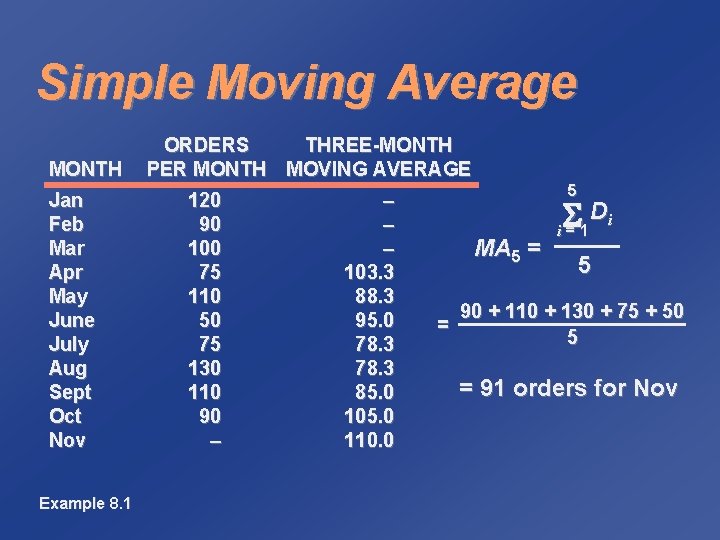
Simple Moving Average MONTH Jan Feb Mar Apr May June July Aug Sept Oct Nov Example 8. 1 ORDERS THREE-MONTH PER MONTH MOVING AVERAGE 120 90 100 75 110 50 75 130 110 90 – – 103. 3 88. 3 95. 0 78. 3 85. 0 105. 0 110. 0 5 MA 5 = = Di i=1 5 90 + 110 + 130 + 75 + 50 5 = 91 orders for Nov

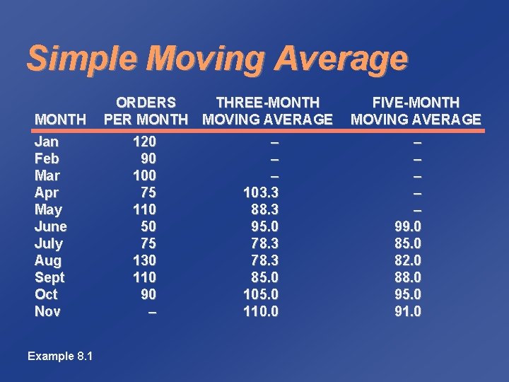
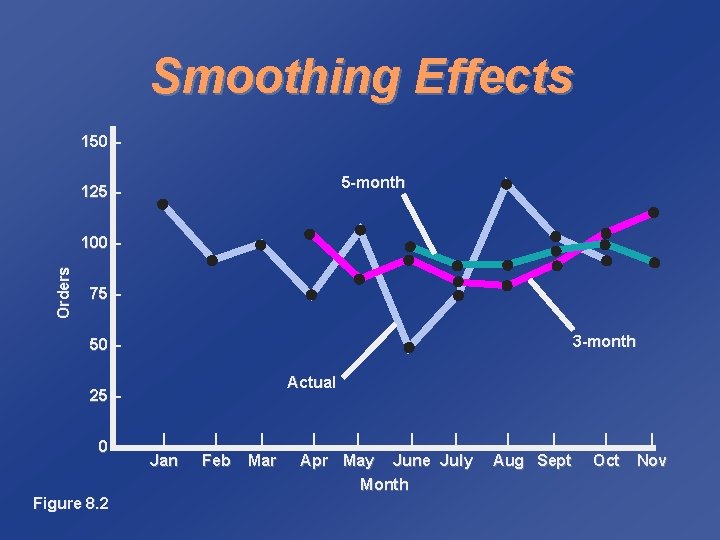
Simple Moving Average MONTH Jan Feb Mar Apr May June July Aug Sept Oct Nov Example 8. 1 ORDERS THREE-MONTH PER MONTH MOVING AVERAGE 120 90 100 75 110 50 75 130 110 90 – – 103. 3 88. 3 95. 0 78. 3 85. 0 105. 0 110. 0 FIVE-MONTH MOVING AVERAGE – – – 99. 0 85. 0 82. 0 88. 0 95. 0 91. 0

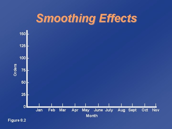
Smoothing Effects 150 – 125 – Orders 100 – 75 – 50 – 25 – 0– Figure 8. 2 | Jan | Feb | Mar | | Apr May June July Month | | Aug Sept | Oct | Nov

Smoothing Effects 150 – 125 – Orders 100 – 75 – 50 – Actual 25 – 0– Figure 8. 2 | Jan | Feb | Mar | | Apr May June July Month | | Aug Sept | Oct | Nov

Smoothing Effects 150 – 125 – Orders 100 – 75 – 3 -month 50 – Actual 25 – 0– Figure 8. 2 | Jan | Feb | Mar | | Apr May June July Month | | Aug Sept | Oct | Nov

Smoothing Effects 150 – 5 -month 125 – Orders 100 – 75 – 3 -month 50 – Actual 25 – 0– Figure 8. 2 | Jan | Feb | Mar | | Apr May June July Month | | Aug Sept | Oct | Nov

Weighted Moving Average ü Adjusts moving average method to more closely reflect data fluctuations

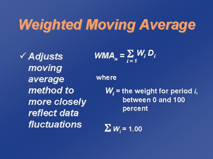
Weighted Moving Average WMAn = Wi Di ü Adjusts i=1 moving where average Wi = the weight for period i, method to between 0 and 100 more closely percent reflect data fluctuations W = 1. 00 i

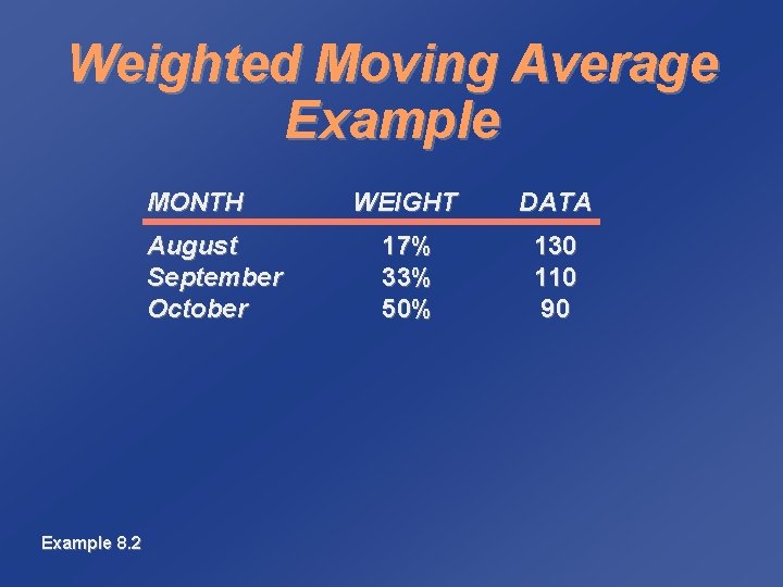
Weighted Moving Average Example MONTH August September October Example 8. 2 WEIGHT DATA 17% 33% 50% 130 110 90

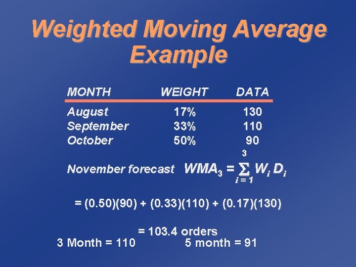
Weighted Moving Average Example MONTH August September October WEIGHT DATA 17% 33% 50% 130 110 90 3 November forecast WMA 3 = Wi Di i=1 = (0. 50)(90) + (0. 33)(110) + (0. 17)(130) = 103. 4 orders 3 Month = 110 5 month = 91

Exponential Smoothing ü Averaging method ü Weights most recent data more strongly ü Reacts more to recent changes ü Widely used, accurate method

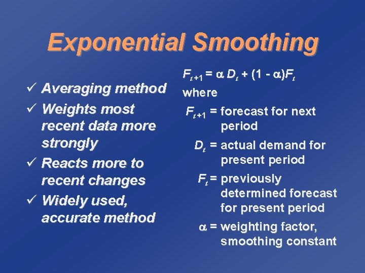
Exponential Smoothing ü Averaging method ü Weights most recent data more strongly ü Reacts more to recent changes ü Widely used, accurate method Ft +1 = Dt + (1 - )Ft where Ft +1 = forecast for next period Dt = actual demand for present period Ft = previously determined forecast for present period = weighting factor, smoothing constant

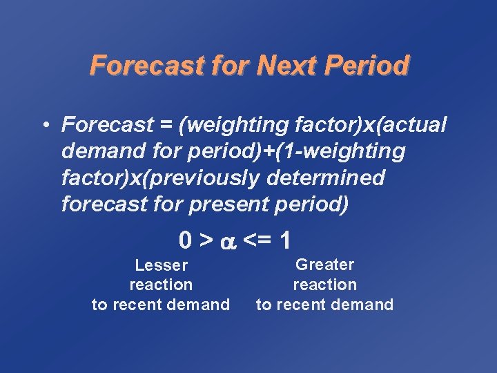
Forecast for Next Period • Forecast = (weighting factor)x(actual demand for period)+(1 -weighting factor)x(previously determined forecast for present period) 0 > <= 1 Lesser reaction to recent demand Greater reaction to recent demand

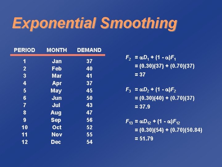
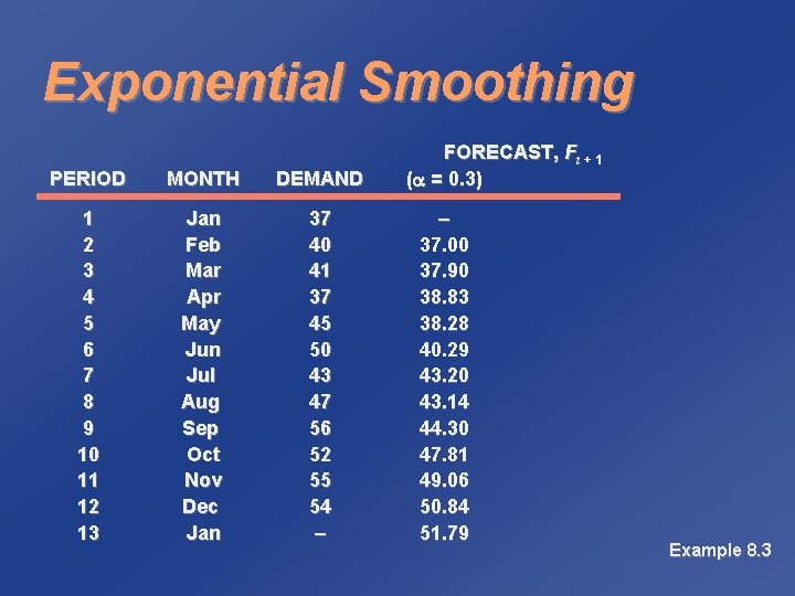
Exponential Smoothing PERIOD MONTH DEMAND 1 2 3 4 5 6 7 8 9 10 11 12 Jan Feb Mar Apr May Jun Jul Aug Sep Oct Nov Dec 37 40 41 37 45 50 43 47 56 52 55 54 F 2 = D 1 + (1 - )F 1 = (0. 30)(37) + (0. 70)(37) = 37 F 3 = D 2 + (1 - )F 2 = (0. 30)(40) + (0. 70)(37) = 37. 9 F 13 = D 12 + (1 - )F 12 = (0. 30)(54) + (0. 70)(50. 84) = 51. 79

Exponential Smoothing PERIOD MONTH DEMAND 1 2 3 4 5 6 7 8 9 10 11 12 13 Jan Feb Mar Apr May Jun Jul Aug Sep Oct Nov Dec Jan 37 40 41 37 45 50 43 47 56 52 55 54 – FORECAST, Ft + 1 ( = 0. 3) – 37. 00 37. 90 38. 83 38. 28 40. 29 43. 20 43. 14 44. 30 47. 81 49. 06 50. 84 51. 79 Example 8. 3

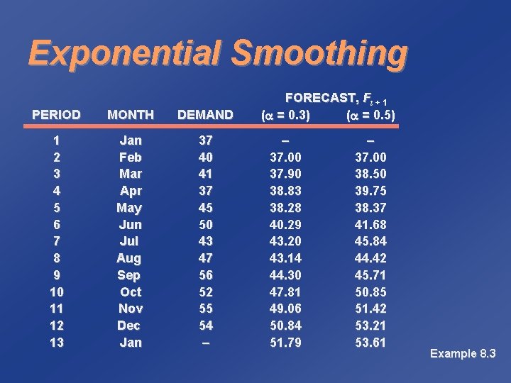
Exponential Smoothing PERIOD MONTH DEMAND 1 2 3 4 5 6 7 8 9 10 11 12 13 Jan Feb Mar Apr May Jun Jul Aug Sep Oct Nov Dec Jan 37 40 41 37 45 50 43 47 56 52 55 54 – FORECAST, Ft + 1 ( = 0. 3) ( = 0. 5) – 37. 00 37. 90 38. 83 38. 28 40. 29 43. 20 43. 14 44. 30 47. 81 49. 06 50. 84 51. 79 – 37. 00 38. 50 39. 75 38. 37 41. 68 45. 84 44. 42 45. 71 50. 85 51. 42 53. 21 53. 61 Example 8. 3

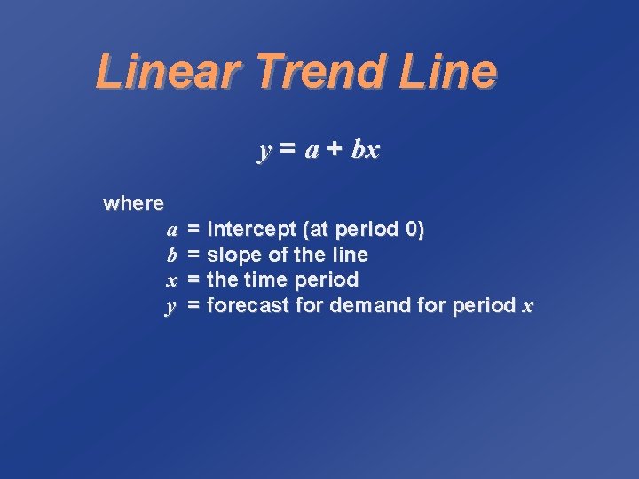
Linear Trend Line y = a + bx where a b x y = intercept (at period 0) = slope of the line = the time period = forecast for demand for period x

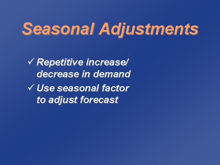
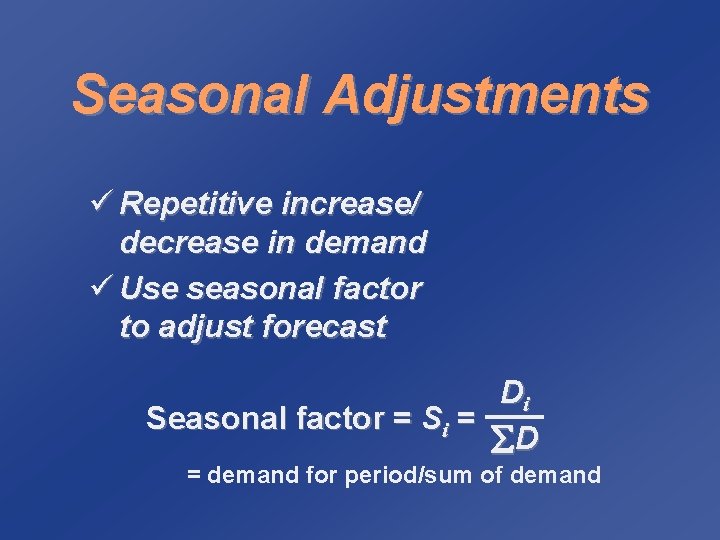
Seasonal Adjustments ü Repetitive increase/ decrease in demand ü Use seasonal factor to adjust forecast

Seasonal Adjustments ü Repetitive increase/ decrease in demand ü Use seasonal factor to adjust forecast Di Seasonal factor = Si = D = demand for period/sum of demand

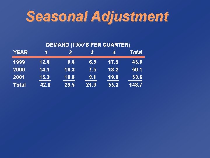
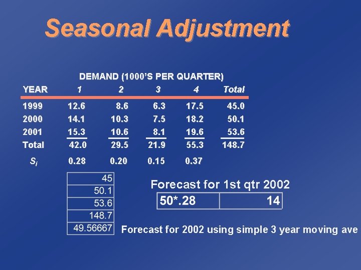
Seasonal Adjustment YEAR 1999 2000 2001 Total DEMAND (1000’S PER QUARTER) 1 2 3 4 Total 12. 6 14. 1 15. 3 42. 0 8. 6 10. 3 10. 6 29. 5 6. 3 7. 5 8. 1 21. 9 17. 5 18. 2 19. 6 55. 3 45. 0 50. 1 53. 6 148. 7

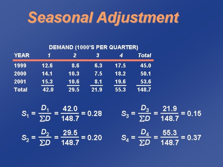
Seasonal Adjustment YEAR 1999 2000 2001 Total DEMAND (1000’S PER QUARTER) 1 2 3 4 Total 12. 6 14. 1 15. 3 42. 0 8. 6 10. 3 10. 6 29. 5 6. 3 7. 5 8. 1 21. 9 17. 5 18. 2 19. 6 55. 3 45. 0 50. 1 53. 6 148. 7 D 1 42. 0 S 1 = = = 0. 28 D 148. 7 D 3 21. 9 S 3 = = = 0. 15 D 148. 7 D 2 29. 5 S 2 = = = 0. 20 D 148. 7 D 4 55. 3 S 4 = = = 0. 37 D 148. 7

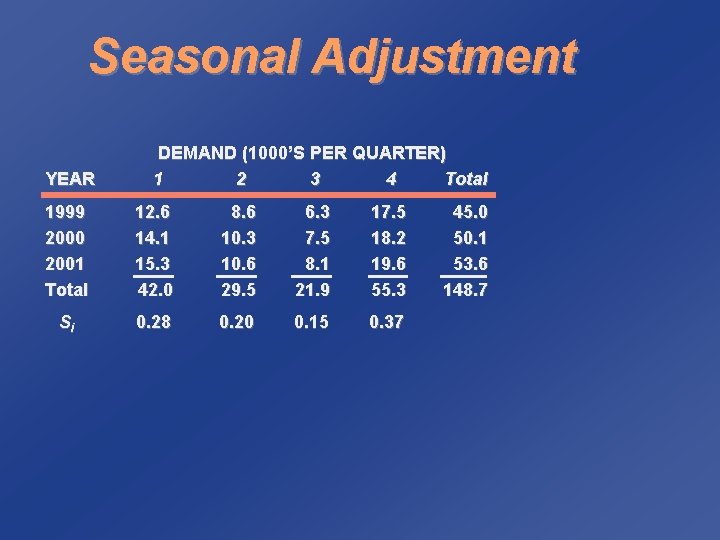
Seasonal Adjustment YEAR DEMAND (1000’S PER QUARTER) 1 2 3 4 Total 1999 2000 2001 Total 12. 6 14. 1 15. 3 42. 0 8. 6 10. 3 10. 6 29. 5 6. 3 7. 5 8. 1 21. 9 17. 5 18. 2 19. 6 55. 3 Si 0. 28 0. 20 0. 15 0. 37 45. 0 50. 1 53. 6 148. 7

Seasonal Adjustment YEAR DEMAND (1000’S PER QUARTER) 1 2 3 4 Total 1999 2000 2001 Total 12. 6 14. 1 15. 3 42. 0 8. 6 10. 3 10. 6 29. 5 6. 3 7. 5 8. 1 21. 9 17. 5 18. 2 19. 6 55. 3 Si 0. 28 0. 20 0. 15 0. 37 45. 0 50. 1 53. 6 148. 7 Forecast for 1 st qtr 2002 Forecast for 2002 using simple 3 year moving ave

Forecast Accuracy ü Find a method which minimizes error ü Error = Actual - Forecast ü Mean Absolute Deviation (MAD)

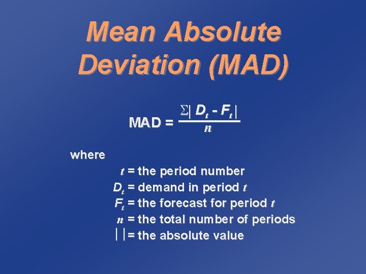
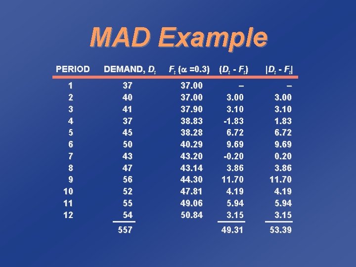
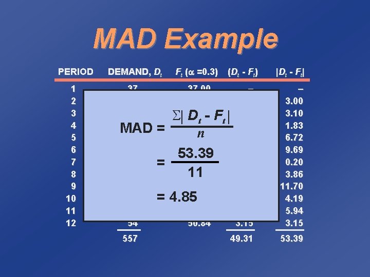
Mean Absolute Deviation (MAD) S Dt - F t MAD = n where t = the period number Dt = demand in period t Ft = the forecast for period t n = the total number of periods = the absolute value

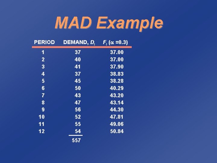
MAD Example PERIOD 1 2 3 4 5 6 7 8 9 10 11 12 DEMAND, Dt Ft ( =0. 3) 37 40 41 37 45 50 43 47 56 52 55 54 37. 00 37. 90 38. 83 38. 28 40. 29 43. 20 43. 14 44. 30 47. 81 49. 06 50. 84 557

MAD Example PERIOD 1 2 3 4 5 6 7 8 9 10 11 12 DEMAND, Dt Ft ( =0. 3) (Dt - Ft) |Dt - Ft| 37 40 41 37 45 50 43 47 56 52 55 54 37. 00 37. 90 38. 83 38. 28 40. 29 43. 20 43. 14 44. 30 47. 81 49. 06 50. 84 – 3. 00 3. 10 -1. 83 6. 72 9. 69 -0. 20 3. 86 11. 70 4. 19 5. 94 3. 15 – 3. 00 3. 10 1. 83 6. 72 9. 69 0. 20 3. 86 11. 70 4. 19 5. 94 3. 15 49. 31 53. 39 557

MAD Example PERIOD 1 2 3 4 5 6 7 8 9 10 11 12 DEMAND, Dt 37 40 41 37 MAD 45 50 43 47 56 52 55 54 557 = = = Ft ( =0. 3) (Dt - Ft) |Dt - Ft| 37. 00 – 37. 00 3. 00 S 37. 90 Dt - Ft 3. 10 38. 83 -1. 83 n 38. 28 6. 72 40. 29 9. 69 53. 39 43. 20 -0. 20 11 43. 14 3. 86 44. 30 11. 70 47. 81 4. 19 4. 85 49. 06 5. 94 50. 84 3. 15 – 3. 00 3. 10 1. 83 6. 72 9. 69 0. 20 3. 86 11. 70 4. 19 5. 94 3. 15 49. 31 53. 39

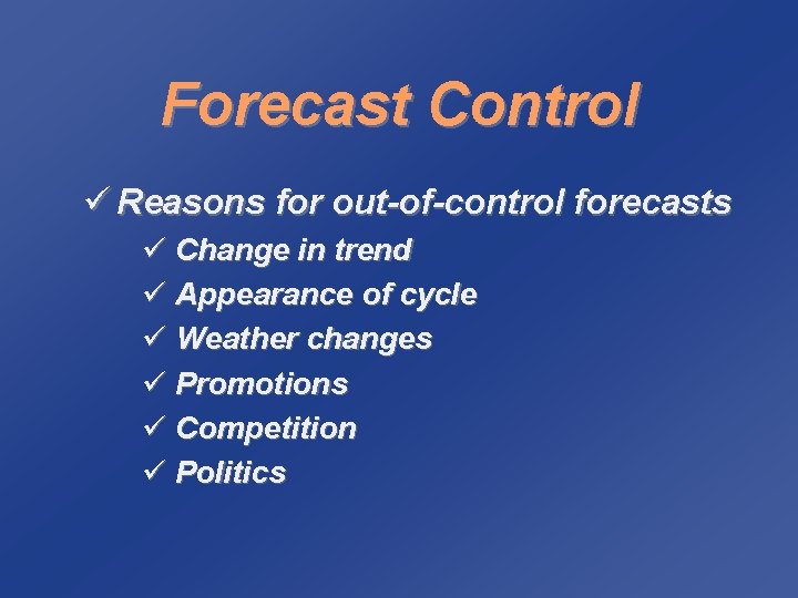
Forecast Control ü Reasons for out-of-control forecasts ü Change in trend ü Appearance of cycle ü Weather changes ü Promotions ü Competition ü Politics

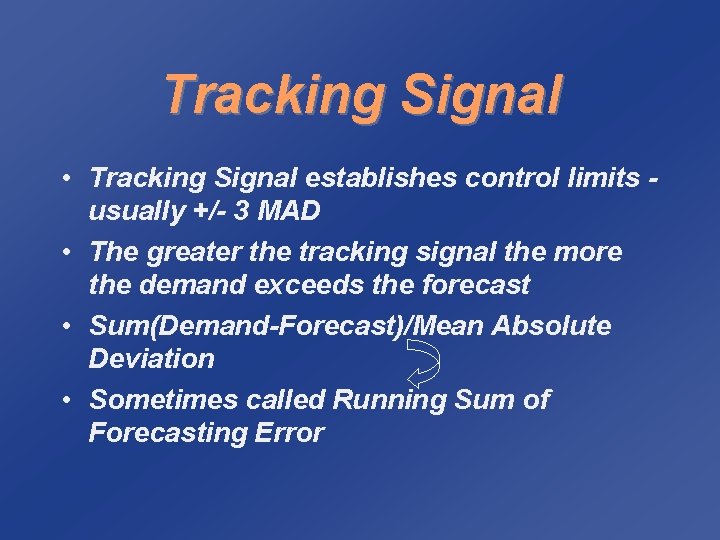
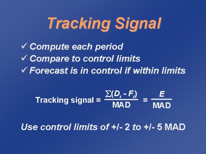
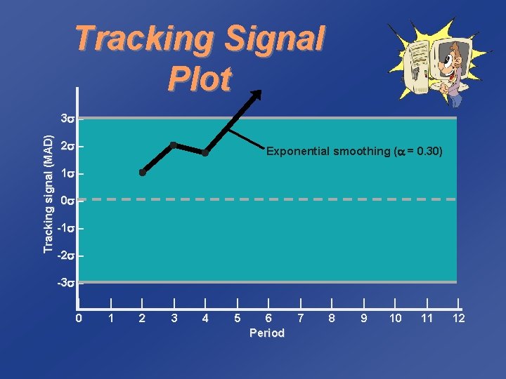
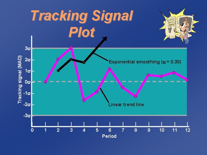
Tracking Signal • Tracking Signal establishes control limits usually +/- 3 MAD • The greater the tracking signal the more the demand exceeds the forecast • Sum(Demand-Forecast)/Mean Absolute Deviation • Sometimes called Running Sum of Forecasting Error

Tracking Signal ü Compute each period ü Compare to control limits ü Forecast is in control if within limits (D t - F t ) E Tracking signal = = MAD Use control limits of +/- 2 to +/- 5 MAD

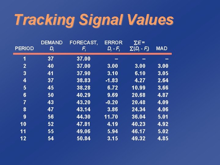
Tracking Signal Values PERIOD DEMAND Dt FORECAST, Ft 1 2 3 4 5 6 7 8 9 10 11 12 37 40 41 37 45 50 43 47 56 52 55 54 37. 00 37. 90 38. 83 38. 28 40. 29 43. 20 43. 14 44. 30 47. 81 49. 06 50. 84 ERROR Dt - F t – 3. 00 3. 10 -1. 83 6. 72 9. 69 -0. 20 3. 86 11. 70 4. 19 5. 94 3. 15 E = (Dt - Ft) MAD – 3. 00 6. 10 4. 27 10. 99 20. 68 20. 48 24. 34 36. 04 40. 23 46. 17 49. 32 – 3. 00 3. 05 2. 64 3. 66 4. 87 4. 09 4. 06 5. 01 4. 92 5. 02 4. 85

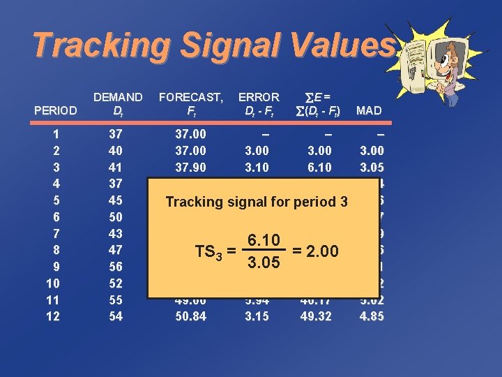
Tracking Signal Values PERIOD DEMAND Dt 1 2 3 4 5 6 7 8 9 10 11 12 37 40 41 37 45 50 43 47 56 52 55 54 FORECAST, Ft ERROR Dt - F t E = (Dt - Ft) 37. 00 – – 37. 00 37. 90 3. 10 6. 10 38. 83 -1. 83 4. 27 38. 28 6. 72 for period 10. 99 3 Tracking signal 40. 29 9. 69 20. 68 43. 20 -0. 20 6. 10 20. 48 43. 14 TS 3 = 3. 86 =24. 34 2. 00 3. 05 36. 04 44. 30 11. 70 47. 81 4. 19 40. 23 49. 06 5. 94 46. 17 50. 84 3. 15 49. 32 MAD – 3. 00 3. 05 2. 64 3. 66 4. 87 4. 09 4. 06 5. 01 4. 92 5. 02 4. 85

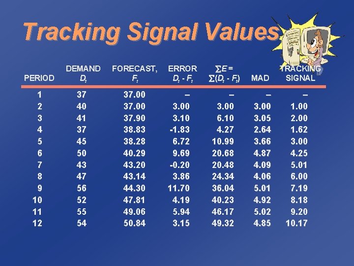
Tracking Signal Values PERIOD DEMAND Dt FORECAST, Ft 1 2 3 4 5 6 7 8 9 10 11 12 37 40 41 37 45 50 43 47 56 52 55 54 37. 00 37. 90 38. 83 38. 28 40. 29 43. 20 43. 14 44. 30 47. 81 49. 06 50. 84 ERROR Dt - F t – 3. 00 3. 10 -1. 83 6. 72 9. 69 -0. 20 3. 86 11. 70 4. 19 5. 94 3. 15 E = (Dt - Ft) MAD – 3. 00 6. 10 4. 27 10. 99 20. 68 20. 48 24. 34 36. 04 40. 23 46. 17 49. 32 – 3. 00 3. 05 2. 64 3. 66 4. 87 4. 09 4. 06 5. 01 4. 92 5. 02 4. 85 TRACKING SIGNAL – 1. 00 2. 00 1. 62 3. 00 4. 25 5. 01 6. 00 7. 19 8. 18 9. 20 10. 17

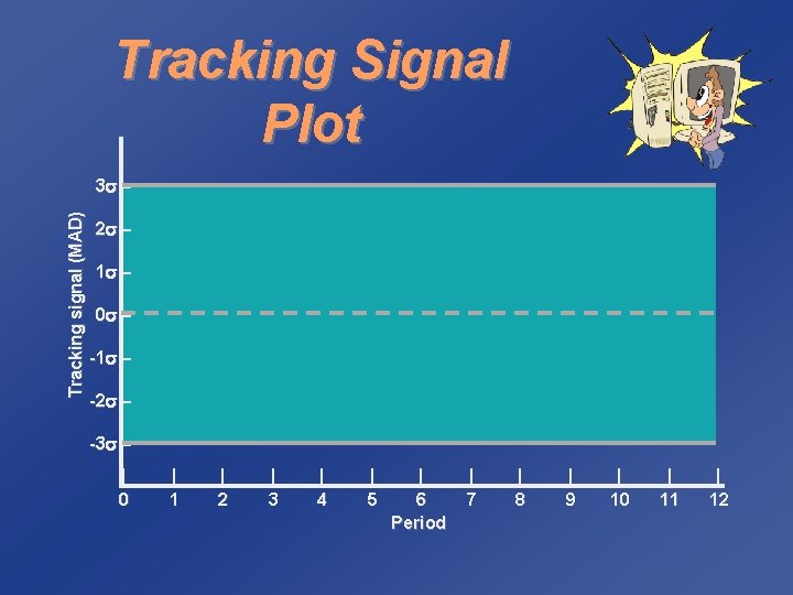
Tracking Signal Plot Tracking signal (MAD) 3 – 2 – 1 – 0 – -1 – -2 – -3 – | 0 | 1 | 2 | 3 | 4 | 5 | 6 Period | 7 | 8 | 9 | 10 | 11 | 12

Tracking Signal Plot Tracking signal (MAD) 3 – 2 – Exponential smoothing ( = 0. 30) 1 – 0 – -1 – -2 – -3 – | 0 | 1 | 2 | 3 | 4 | 5 | 6 Period | 7 | 8 | 9 | 10 | 11 | 12

Tracking Signal Plot Tracking signal (MAD) 3 – 2 – Exponential smoothing ( = 0. 30) 1 – 0 – -1 – -2 – Linear trend line -3 – | 0 | 1 | 2 | 3 | 4 | 5 | 6 Period | 7 | 8 | 9 | 10 | 11 | 12

Forecasting • Long Term – location, capacity, new product design • Short Term – production, inventory control, labor levels, cost controls Questions?

Next Week • Chap 6 • Chapter 12