Chapter 15 Pricing and Revenue Management in the

Chapter 15 Pricing and Revenue Management in the Supply Chain Copyright © 2010 Pearson Education, Inc. Publishing as Prentice Hall. 15 -1

Outline u The Role of Pricing and Revenue Management in a Supply Chain u Pricing and Revenue Management for Multiple Customer Segments u Pricing and Revenue Management for Perishable Assets u Pricing and Revenue Management for Seasonable Demand u Pricing and Revenue Management for Bulk and Spot Customers u The Role of IT in Pricing and Revenue Management u Using Pricing and Revenue Management in Practice u Summary of Learning Objectives Copyright © 2010 Pearson Education, Inc. Publishing as Prentice Hall. 15 -2

The Role of Pricing and Revenue Management in the Supply Chain u. Revenue management is the use of pricing to increase the profit generated from a limited supply of supply chain assets u. Supply assets exist in two forms: capacity and inventory u. Revenue management may also be defined as the use of differential pricing based on customer segment, time of use, and product or capacity availability to increase supply chain profits u. Most common example is probably in airline pricing Copyright © 2010 Pearson Education, Inc. Publishing as Prentice Hall. 15 -3

Conditions Under Which Revenue Management Has the Greatest Effect u. The value of the product varies in different market segments (Example: airline seats) u. The product is highly perishable or product waste occurs (Example: fashion and seasonal apparel) u. Demand has seasonal and other peaks (Example: products ordered at Amazon. com) u. The product is sold both in bulk and on the spot market (Example: owner of warehouse who can decide whether to lease the entire warehouse through long-term contracts or save a portion of the warehouse for use in the spot market) Copyright © 2010 Pearson Education, Inc. Publishing as Prentice Hall. 15 -4

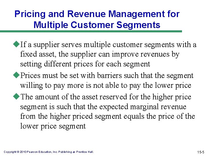
Pricing and Revenue Management for Multiple Customer Segments u. If a supplier serves multiple customer segments with a fixed asset, the supplier can improve revenues by setting different prices for each segment u. Prices must be set with barriers such that the segment willing to pay more is not able to pay the lower price u. The amount of the asset reserved for the higher price segment is such that the expected marginal revenue from the higher priced segment equals the price of the lower price segment Copyright © 2010 Pearson Education, Inc. Publishing as Prentice Hall. 15 -5

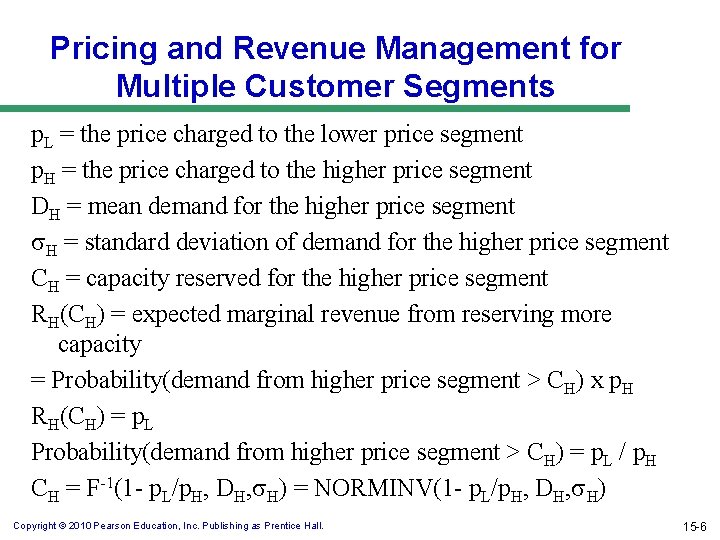
Pricing and Revenue Management for Multiple Customer Segments p. L = the price charged to the lower price segment p. H = the price charged to the higher price segment DH = mean demand for the higher price segment s. H = standard deviation of demand for the higher price segment CH = capacity reserved for the higher price segment RH(CH) = expected marginal revenue from reserving more capacity = Probability(demand from higher price segment > CH) x p. H RH(CH) = p. L Probability(demand from higher price segment > CH) = p. L / p. H CH = F-1(1 - p. L/p. H, DH, s. H) = NORMINV(1 - p. L/p. H, DH, s. H) Copyright © 2010 Pearson Education, Inc. Publishing as Prentice Hall. 15 -6

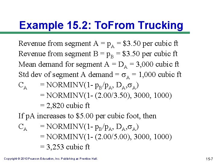
Example 15. 2: To. From Trucking Revenue from segment A = p. A = $3. 50 per cubic ft Revenue from segment B = p. B = $3. 50 per cubic ft Mean demand for segment A = DA = 3, 000 cubic ft Std dev of segment A demand = s. A = 1, 000 cubic ft CA = NORMINV(1 - p. B/p. A, DA, s. A) = NORMINV(1 - (2. 00/3. 50), 3000, 1000) = 2, 820 cubic ft If p. A increases to $5. 00 per cubic foot, then CA = NORMINV(1 - p. B/p. A, DA, s. A) = NORMINV(1 - (2. 00/5. 00), 3000, 1000) = 3, 253 cubic ft Copyright © 2010 Pearson Education, Inc. Publishing as Prentice Hall. 15 -7

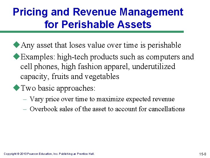
Pricing and Revenue Management for Perishable Assets u. Any asset that loses value over time is perishable u. Examples: high-tech products such as computers and cell phones, high fashion apparel, underutilized capacity, fruits and vegetables u. Two basic approaches: – Vary price over time to maximize expected revenue – Overbook sales of the asset to account for cancellations Copyright © 2010 Pearson Education, Inc. Publishing as Prentice Hall. 15 -8

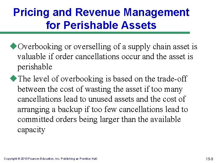
Pricing and Revenue Management for Perishable Assets u. Overbooking or overselling of a supply chain asset is valuable if order cancellations occur and the asset is perishable u. The level of overbooking is based on the trade-off between the cost of wasting the asset if too many cancellations lead to unused assets and the cost of arranging a backup if too few cancellations lead to committed orders being larger than the available capacity Copyright © 2010 Pearson Education, Inc. Publishing as Prentice Hall. 15 -9

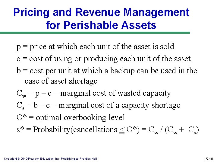
Pricing and Revenue Management for Perishable Assets p = price at which each unit of the asset is sold c = cost of using or producing each unit of the asset b = cost per unit at which a backup can be used in the case of asset shortage Cw = p – c = marginal cost of wasted capacity Cs = b – c = marginal cost of a capacity shortage O* = optimal overbooking level s* = Probability(cancellations < O*) = Cw / (Cw + Cs) Copyright © 2010 Pearson Education, Inc. Publishing as Prentice Hall. 15 -10

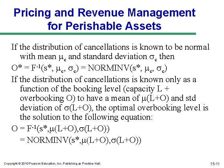
Pricing and Revenue Management for Perishable Assets If the distribution of cancellations is known to be normal with mean mc and standard deviation sc then O* = F-1(s*, mc, sc) = NORMINV(s*, mc, sc) If the distribution of cancellations is known only as a function of the booking level (capacity L + overbooking O) to have a mean of m(L+O) and std deviation of s(L+O), the optimal overbooking level is the solution to the following equation: O = F-1(s*, m(L+O), s(L+O)) = NORMINV(s*, m(L+O), s(L+O)) Copyright © 2010 Pearson Education, Inc. Publishing as Prentice Hall. 15 -11

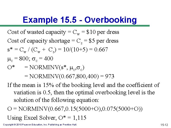
Example 15. 5 - Overbooking Cost of wasted capacity = Cw = $10 per dress Cost of capacity shortage = Cs = $5 per dress s* = Cw / (Cw + Cs) = 10/(10+5) = 0. 667 mc = 800; sc = 400 O* = NORMINV(s*, mc, sc) = NORMINV(0. 667, 800, 400) = 973 If the mean is 15% of the booking level and the coefficient of variation is 0. 5, then the optimal overbooking level is the solution of the following equation: O = NORMINV(0. 667, 0. 15(5000+O), 0. 075(5000+O)) Using Excel Solver, O* = 1, 115 Copyright © 2010 Pearson Education, Inc. Publishing as Prentice Hall. 15 -12

Pricing and Revenue Management for Seasonal Demand u. Seasonal peaks of demand are common in many supply chains u. Examples: Most retailers achieve a large portion of total annual demand in December (Amazon. com) u. Off-peak discounting can shift demand from peak to non-peak periods u. Charge higher price during peak periods and a lower price during off-peak periods Copyright © 2010 Pearson Education, Inc. Publishing as Prentice Hall. 15 -13

Pricing and Revenue Management for Bulk and Spot Customers u Most consumers of production, warehousing, and transportation assets in a supply chain face the problem of constructing a portfolio of long-term bulk contracts and short-term spot market contracts u The basic decision is the size of the bulk contract u The fundamental trade-off is between wasting a portion of the low-cost bulk contract and paying more for the asset on the spot market u Given that both the spot market price and the purchaser’s need for the asset are uncertain, a decision tree approach as discussed in Chapter 6 should be used to evaluate the amount of long-term bulk contract to sign Copyright © 2010 Pearson Education, Inc. Publishing as Prentice Hall. 15 -14

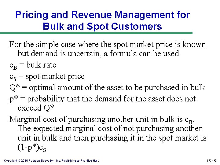
Pricing and Revenue Management for Bulk and Spot Customers For the simple case where the spot market price is known but demand is uncertain, a formula can be used c. B = bulk rate c. S = spot market price Q* = optimal amount of the asset to be purchased in bulk p* = probability that the demand for the asset does not exceed Q* Marginal cost of purchasing another unit in bulk is c. B. The expected marginal cost of not purchasing another unit in bulk and then purchasing it in the spot market is (1 -p*)c. S. Copyright © 2010 Pearson Education, Inc. Publishing as Prentice Hall. 15 -15

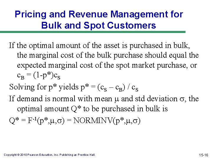
Pricing and Revenue Management for Bulk and Spot Customers If the optimal amount of the asset is purchased in bulk, the marginal cost of the bulk purchase should equal the expected marginal cost of the spot market purchase, or c. B = (1 -p*)c. S Solving for p* yields p* = (c. S – c. B) / c. S If demand is normal with mean m and std deviation s, the optimal amount Q* to be purchased in bulk is Q* = F-1(p*, m, s) = NORMINV(p*, m, s) Copyright © 2010 Pearson Education, Inc. Publishing as Prentice Hall. 15 -16

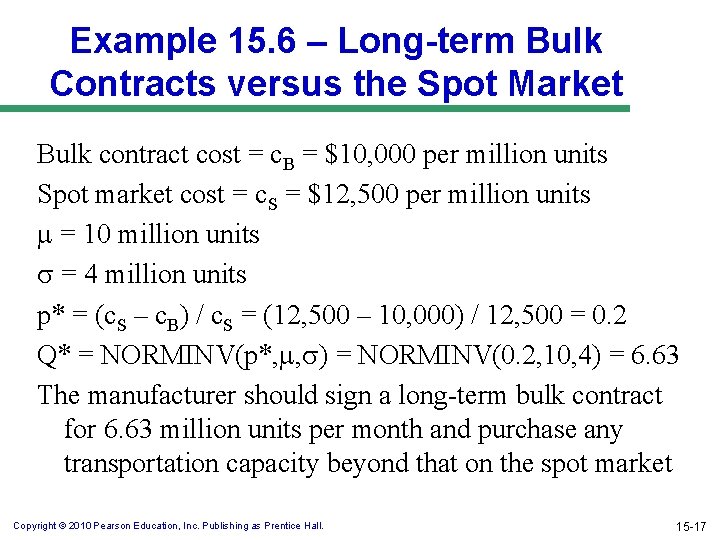
Example 15. 6 – Long-term Bulk Contracts versus the Spot Market Bulk contract cost = c. B = $10, 000 per million units Spot market cost = c. S = $12, 500 per million units m = 10 million units s = 4 million units p* = (c. S – c. B) / c. S = (12, 500 – 10, 000) / 12, 500 = 0. 2 Q* = NORMINV(p*, m, s) = NORMINV(0. 2, 10, 4) = 6. 63 The manufacturer should sign a long-term bulk contract for 6. 63 million units per month and purchase any transportation capacity beyond that on the spot market Copyright © 2010 Pearson Education, Inc. Publishing as Prentice Hall. 15 -17

The Role of IT in Pricing and Revenue Management u. Pricing of perishable assets u. Pricing of retail goods in the consumer packagedgoods category u. Mark downs of goods as the styles and seasons change u. Linking with other areas and applications Copyright © 2010 Pearson Education, Inc. Publishing as Prentice Hall. 15 -18

Using Pricing and Revenue Management in Practice u. Evaluate your market carefully u. Quantify the benefits of revenue management u. Implement a forecasting process u. Apply optimization to obtain the revenue management decision u. Involve both sales and operations u. Understand inform the customer u. Integrate supply planning with revenue management Copyright © 2010 Pearson Education, Inc. Publishing as Prentice Hall. 15 -19

Summary of Learning Objectives u. What is the role of revenue management in a supply chain? u. Under what conditions are revenue management tactics effective? u. What are the trade-offs that must be considered when making revenue management decisions? Copyright © 2010 Pearson Education, Inc. Publishing as Prentice Hall. 15 -20