LESSON 6 SUPPLY CHAIN MANAGEMENT Outline Supply Chain

LESSON 6: SUPPLY CHAIN MANAGEMENT Outline • Supply Chain and Supply Chain Management • Supply Chain Database and Planning • Supply Chain Management and Competitive Advantage • Investment in Supply Chain • Transportation Problem 1

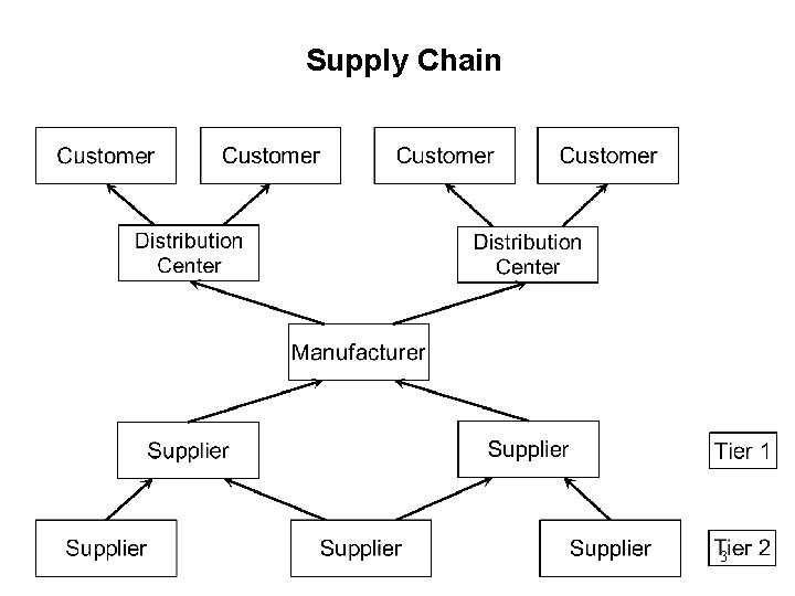
Supply Chain • A supply chain represents all the stages at which value is added in producing and delivering a product or service from suppliers (and their suppliers) to customers (and their customers). • A conceptual view of the supply chain network is shown on the next slide. In practice, the supply chain network can be quite large and complex. 2

Supply Chain 3

Supply Chain Management • Supply chain management is the coordination of the following functions and activities along the supply chain: – Planning and managing of supply and demand – Acquiring material – Warehousing – Inventory control and distribution – Producing and scheduling the product or service – Delivery and customer service 4

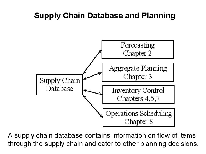
Supply Chain Database and Planning A supply chain database contains information on flow of items 5 through the supply chain and cater to other planning decisions.

Supply Chain Management and Competitive Advantage • Competitive advantage may be obtained with a total systems approach to managing flow of information, materials and services along the supply chain • Text p. 307 discusses how Wal-Mart obtained a competitive advantage and won market-share over KMart with an investment in information technology towards an efficient supply chain management. 6

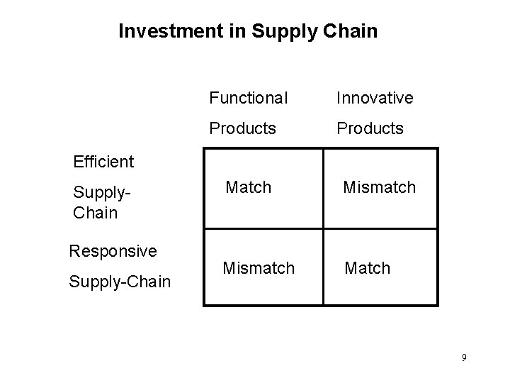
Investment in Supply Chain • For high profit margin (high tech products, innovative products) products, it’s important to create a responsive supply chain. The goals of investment are: – Reduce stockout – Reduce lead time along the supply chain 7

Investment in Supply Chain • For low profit margin (staple products, functional products) products, it’s important to create an efficient supply chain. The goals of investment are: – Reduce cost – Increase resource utilization, minimize inventory, – select vendors on the basis of cost and quality, design products that can be produced depending on such vendors 8

Investment in Supply Chain Functional Innovative Products Efficient Supply. Chain Responsive Supply-Chain Match Mismatch Match 9

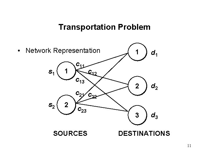
Transportation Problem • The transportation problem minimizes the total shipping costs of transporting goods from m origins (each with a supply si) to n destinations (each with a demand dj), when the unit shipping cost from an origin, i, to a destination, j, is cij. • The network representation for a transportation problem with two sources and three destinations is given on the next slide. 10

Transportation Problem • Network Representation s 1 1 c 13 2 c 23 SOURCES d 1 2 d 2 3 d 3 c 12 c 21 c 22 s 2 1 DESTINATIONS 11

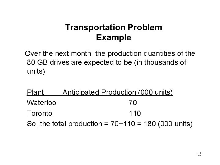
Transportation Problem Example The Riverside Disk Drive Corporation produces Ambassador drives for personal computers in two plants located in Waterloo and Toronto. Periodically, shipments are made from these production facilities to three warehouses located in Windsor, London, and Ottawa. 12

Transportation Problem Example Over the next month, the production quantities of the 80 GB drives are expected to be (in thousands of units) Plant Anticipated Production (000 units) Waterloo 70 Toronto 110 So, the total production = 70+110 = 180 (000 units) 13

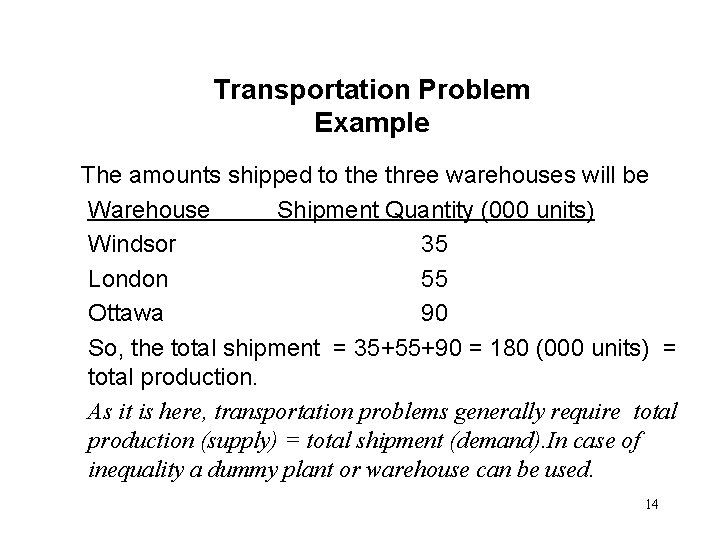
Transportation Problem Example The amounts shipped to the three warehouses will be Warehouse Shipment Quantity (000 units) Windsor 35 London 55 Ottawa 90 So, the total shipment = 35+55+90 = 180 (000 units) = total production. As it is here, transportation problems generally require total production (supply) = total shipment (demand). In case of inequality a dummy plant or warehouse can be used. 14

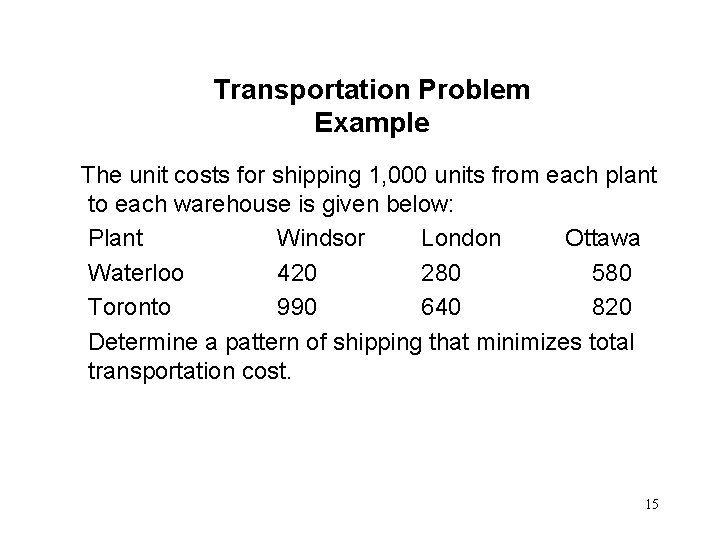
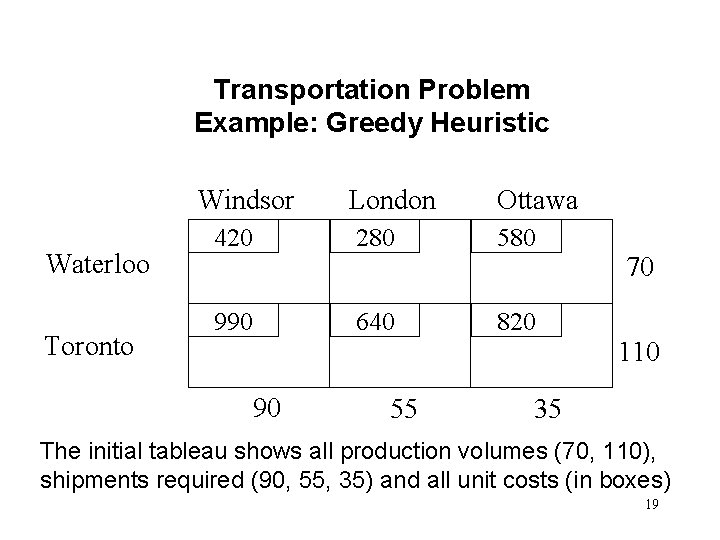
Transportation Problem Example The unit costs for shipping 1, 000 units from each plant to each warehouse is given below: Plant Windsor London Ottawa Waterloo 420 280 580 Toronto 990 640 820 Determine a pattern of shipping that minimizes total transportation cost. 15

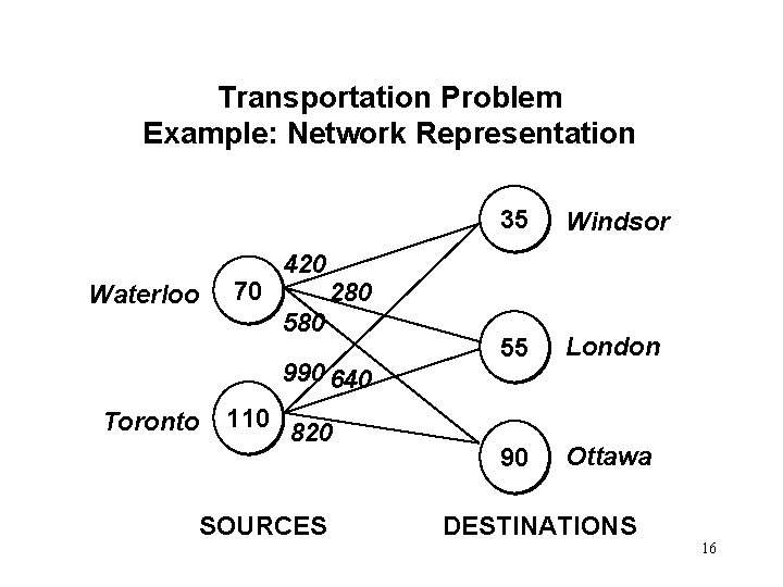
Transportation Problem Example: Network Representation Waterloo 70 420 580 110 820 SOURCES Windsor 55 London 90 Ottawa 280 990 640 Toronto 35 DESTINATIONS 16

Transportation Problem A Greedy Heuristic • The transportation problem will be solved using a greedy heuristic and Excel Solver. • The heuristic is easy to use, but does not guarantee an optimal solution. The heuristic provides an intuition on the structure of the problem. • An optimal solution can be obtained by solving the problem as a linear programming problem. Excel Solver will be used to solve the linear programming problem. 17

Transportation Problem A Greedy Heuristic • The greedy heuristic discussed here is an iterative approach. • In each iteration, a minimum unit cost transportation alternative is chosen and the maximum possible units is transported using that alternative. • Note that the maximum units to transport is actually minimum of production available and shipment required. 18

Transportation Problem Example: Greedy Heuristic Windsor Waterloo Toronto London Ottawa 420 280 580 990 640 820 90 55 70 110 35 The initial tableau shows all production volumes (70, 110), shipments required (90, 55, 35) and all unit costs (in boxes) 19

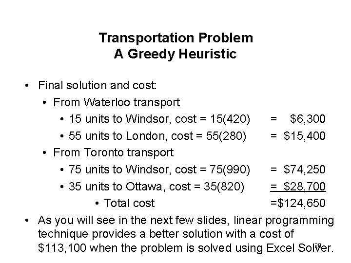
Transportation Problem A Greedy Heuristic • Final solution and cost: • From Waterloo transport • 15 units to Windsor, cost = 15(420) = $6, 300 • 55 units to London, cost = 55(280) = $15, 400 • From Toronto transport • 75 units to Windsor, cost = 75(990) = $74, 250 • 35 units to Ottawa, cost = 35(820) = $28, 700 • Total cost =$124, 650 • As you will see in the next few slides, linear programming technique provides a better solution with a cost of 20 $113, 100 when the problem is solved using Excel Solver.

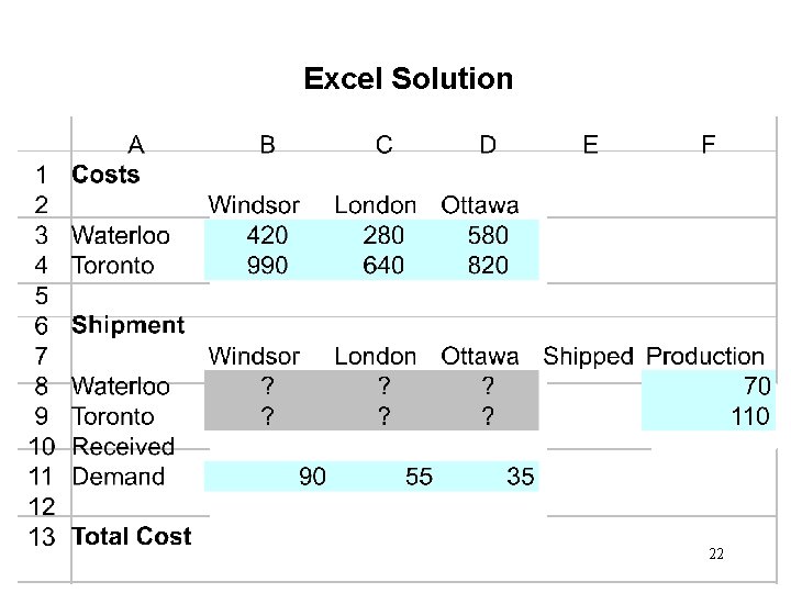
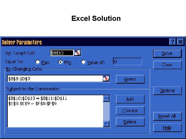
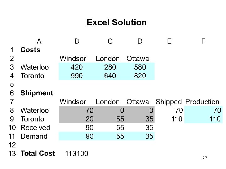
Excel Solution • Set up the spreadsheet as shown on the next slide. • The cells with question marks are the decision variables. Excel will find numbers to these cells. • The cells with numbers are input cells. • Blank cells B 10, C 10, D 10, E 8 and E 9 are to be filled up by formula. Cell B 10 will contain total amount shipped to Windsor as suggested by the Excel solution. So, the formula for this cell is =B 8+B 9. Similarly, C 10 and D 10 will contain total amount shipped to London and Ottawa respectively. Cells E 8 and E 9 will contain total amount shipped from Waterloo and Toronto respectively. All the formula of these cells are listed on Slide 27. 21

Excel Solution 22

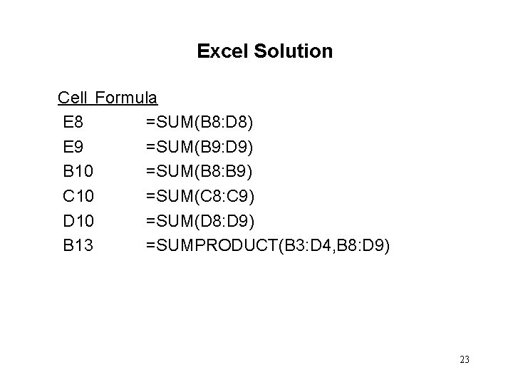
Excel Solution Cell Formula E 8 =SUM(B 8: D 8) E 9 =SUM(B 9: D 9) B 10 =SUM(B 8: B 9) C 10 =SUM(C 8: C 9) D 10 =SUM(D 8: D 9) B 13 =SUMPRODUCT(B 3: D 4, B 8: D 9) 23

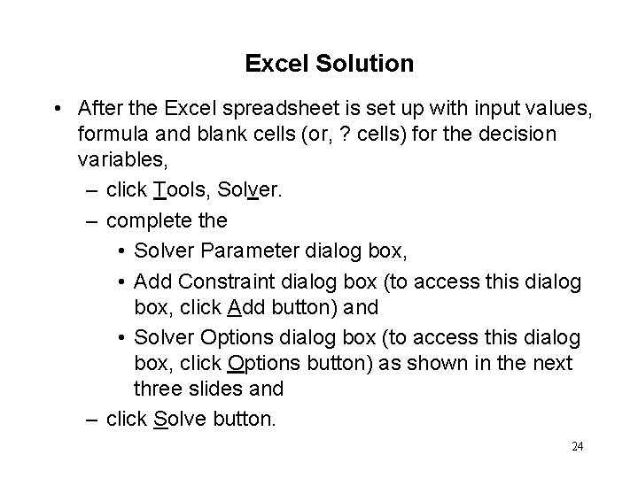
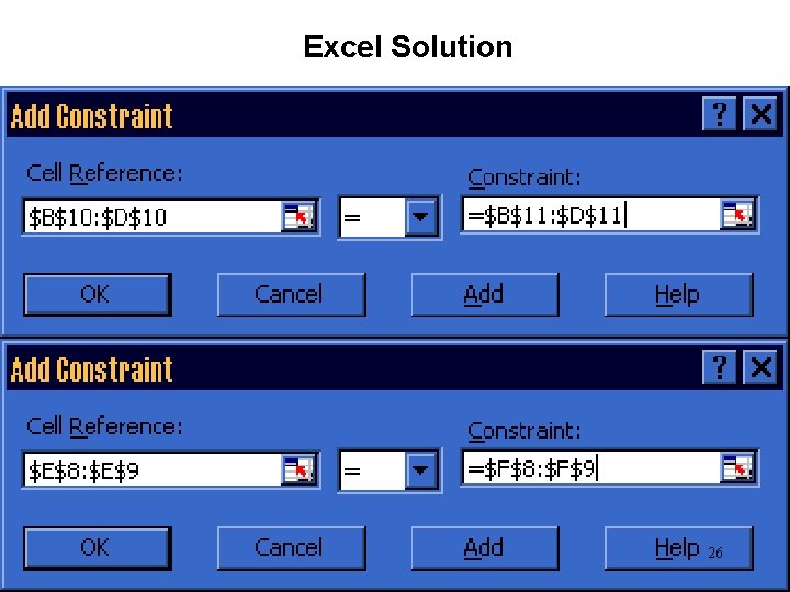
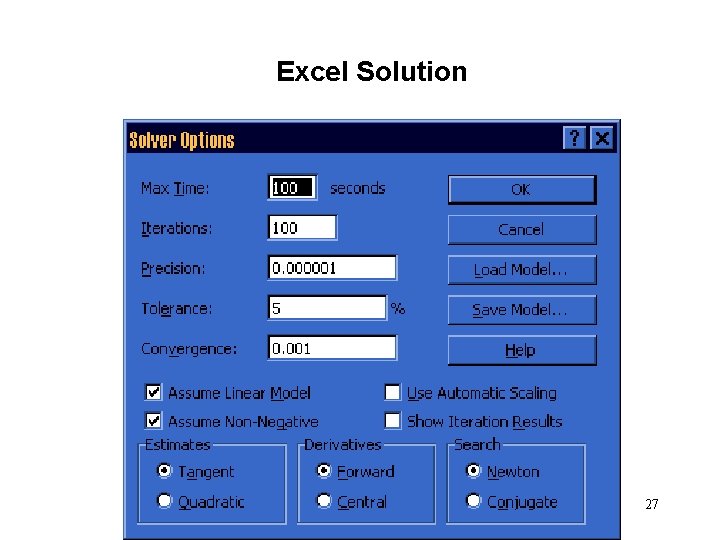
Excel Solution • After the Excel spreadsheet is set up with input values, formula and blank cells (or, ? cells) for the decision variables, – click Tools, Solver. – complete the • Solver Parameter dialog box, • Add Constraint dialog box (to access this dialog box, click Add button) and • Solver Options dialog box (to access this dialog box, click Options button) as shown in the next three slides and – click Solve button. 24

Excel Solution 25

Excel Solution 26

Excel Solution 27

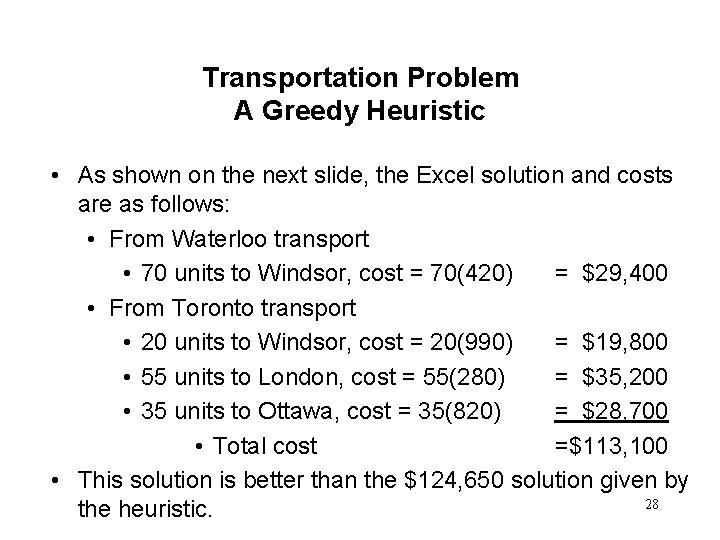
Transportation Problem A Greedy Heuristic • As shown on the next slide, the Excel solution and costs are as follows: • From Waterloo transport • 70 units to Windsor, cost = 70(420) = $29, 400 • From Toronto transport • 20 units to Windsor, cost = 20(990) = $19, 800 • 55 units to London, cost = 55(280) = $35, 200 • 35 units to Ottawa, cost = 35(820) = $28, 700 • Total cost =$113, 100 • This solution is better than the $124, 650 solution given by 28 the heuristic.

Excel Solution 29

READING AND EXERCISES Lesson 6 Reading: – Section 6. 1 pp. 305 -312 (4 th Ed. ), pp. 294 -303 (5 th Ed. ) Exercises: – 6. 1 pp. 319 -320 (4 th Ed. ), p. 310 (5 th Ed. ) 30

LESSON 7: VEHICLE SCHEDULING Outline • • • Vehicle Scheduling Problem Savings Matrix Method Identify Distance Matrix Identify Savings Matrix Rank Savings Assign Customers to Vehicles Sequence Customers within Routes Construction and Improvement Procedures Example 31

Vehicle Scheduling Problem • Goods and items are delivered from one city to another, one province to another and one country to another. In this lesson, we shall discuss a procedure used to deliver items by a fleet of vehicles. • Suppose that a company owns several trucks. The company needs to deliver items to various customers within the Windsor City. The manager takes a map of the city, plots all the customers on the map and finds that the customers are scattered over the entire Windsor area. 32

Vehicle Scheduling Problem • The manager finds that two vehicles will provide a sufficient capacity for all orders. One vehicle will serve the East side and the other the West side. To find out if each vehicle will be able to finish all the deliveries before their due dates, the manager first needs a possible route of each vehicle. Different route provides a different speed limit and risk levels. The manager draws a fast and safe route for each vehicle and estimates delivery times. It turns out that a large number of customers would receive their orders late. 33

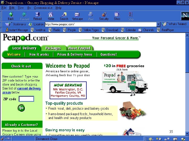
Vehicle Scheduling Problem • The manager then repeats the process with three vehicles, one to the South side, one to the East side, and one to the West side. This plan appeared suitable to meet all the due dates. • Such problems may appear in case of e. g. , an on-line grocery stores such as http: //www. peapod. com. See the next slide for a picture of their website. The orders are taken 24 hours on-line. When the manager starts working in the morning, the manager has to decide number of vehicles and their routes. 34

35

Vehicle Scheduling Problem • Assume that – There are orders from 5 different customers – There are 2 trucks each capable of carrying 200 units 36

Vehicle Scheduling Problem • The manager must solve two sub-problems 1. Split the city into several smaller regions, each of which will be served by one vehicle. This can be done by considering a customer first, assigning the customer to a vehicle, and then assigning other nearby customers to the same vehicle. So, this sub-problem will be called assigning customers to vehicles. 2. Sequence customers served by the same vehicle. 37

Vehicle Scheduling Problem • The objectives of the vehicle scheduling problem can be many. • Following are some examples: – Minimize number of vehicles required – Minimize total distance traveled – Minimize total travel time – Minimize cost • We shall consider the problem with the objective of minimizing total distance. 38

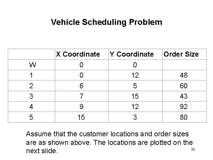
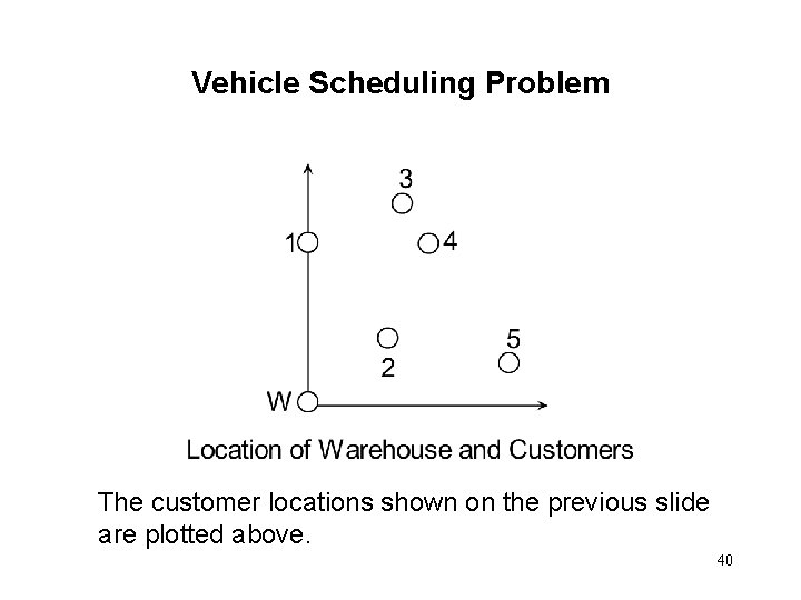
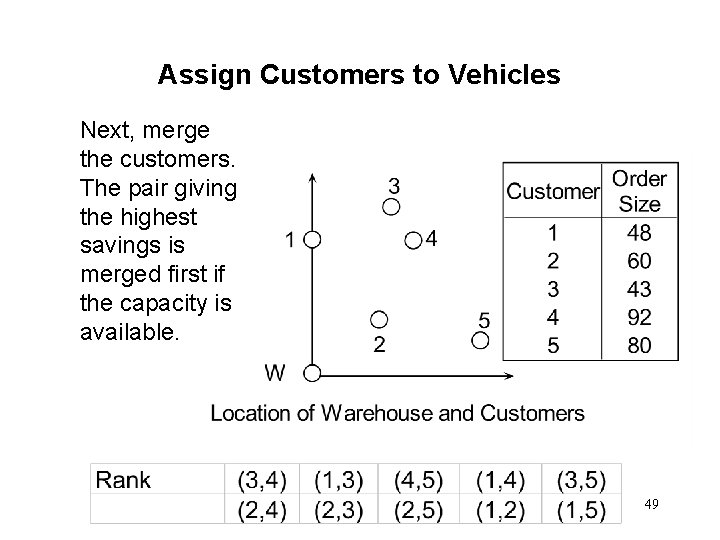
Vehicle Scheduling Problem X Coordinate W 1 2 3 4 5 0 0 6 7 9 15 Y Coordinate 0 12 5 15 12 3 Order Size 48 60 43 92 80 Assume that the customer locations and order sizes are as shown above. The locations are plotted on the 39 next slide.

Vehicle Scheduling Problem The customer locations shown on the previous slide are plotted above. 40

Savings Matrix Method • Following are the steps of the Savings Matrix Method: 1. Identify distance matrix 2. Identify savings Matrix 3. Rank savings 4. Assign customers to vehicles 5. Sequence customers within routes 41

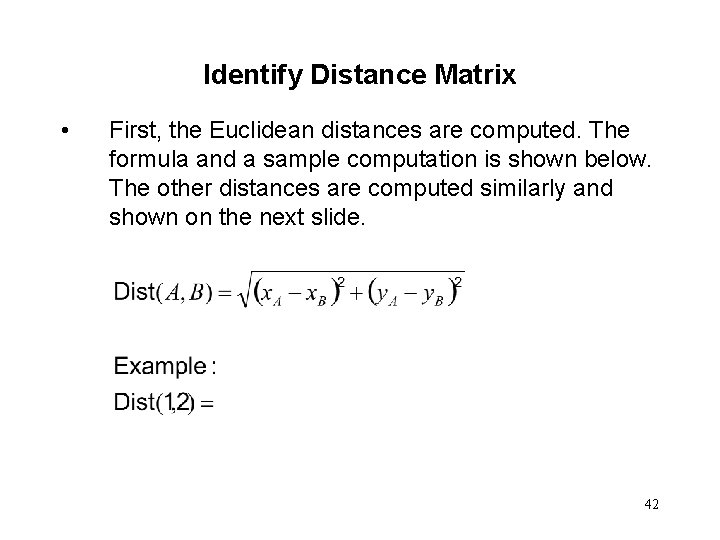
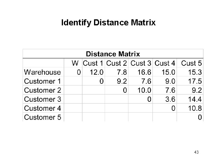
Identify Distance Matrix • First, the Euclidean distances are computed. The formula and a sample computation is shown below. The other distances are computed similarly and shown on the next slide. 42

Identify Distance Matrix 43

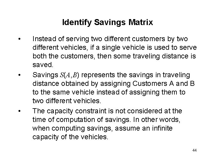
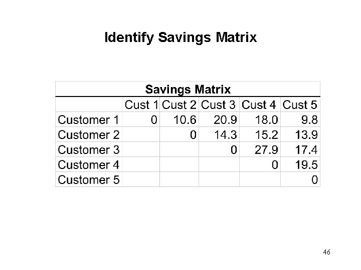
Identify Savings Matrix • • • Instead of serving two different customers by two different vehicles, if a single vehicle is used to serve both the customers, then some traveling distance is saved. Savings S(A, B) represents the savings in traveling distance obtained by assigning Customers A and B to the same vehicle instead of assigning them to two different vehicles. The capacity constraint is not considered at the time of computation of savings. In other words, when computing savings, assume an infinite capacity of the vehicles. 44

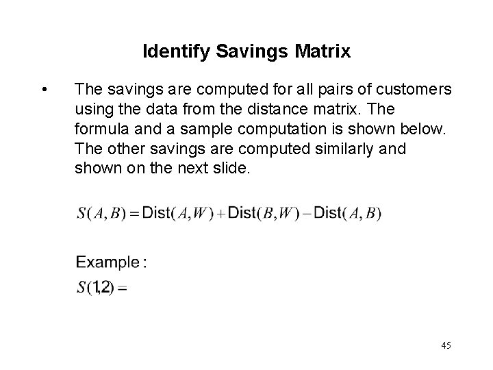
Identify Savings Matrix • The savings are computed for all pairs of customers using the data from the distance matrix. The formula and a sample computation is shown below. The other savings are computed similarly and shown on the next slide. 45

Identify Savings Matrix 46

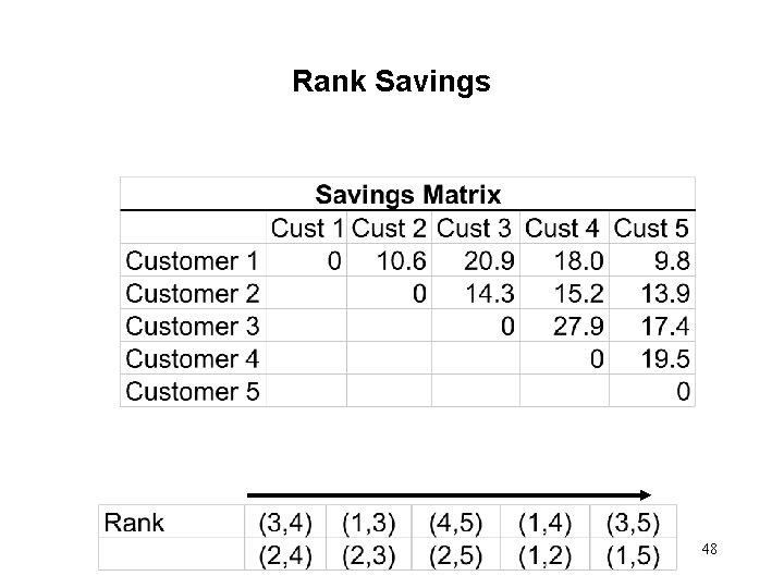
Rank Savings • • • The next step is to rank the savings. The idea is to merge those two customers to the same vehicle, whose merging gives the highest savings. The savings are ranked from high to low. From the savings matrix shown on the previous slide, the highest savings of 27. 9 is obtained by merging Customers 3 and 4 to the same vehicle. Next highest savings of 20. 9 is obtained by merging Customers 1 and 3 to the same vehicle. Similarly the other savings are ranked and shown on the next slide. 47

Rank Savings 48

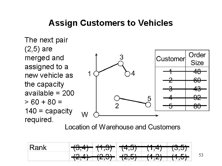
Assign Customers to Vehicles Next, merge the customers. The pair giving the highest savings is merged first if the capacity is available. 49

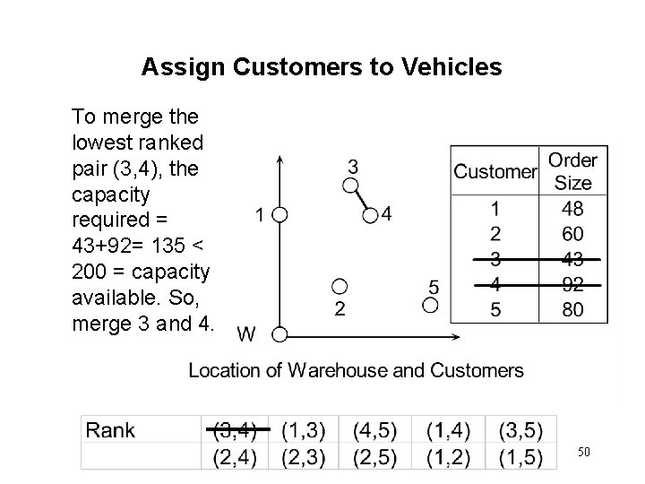
Assign Customers to Vehicles To merge the lowest ranked pair (3, 4), the capacity required = 43+92= 135 < 200 = capacity available. So, merge 3 and 4. 50

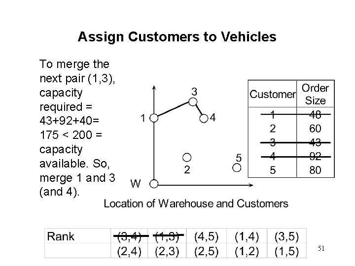
Assign Customers to Vehicles To merge the next pair (1, 3), capacity required = 43+92+40= 175 < 200 = capacity available. So, merge 1 and 3 (and 4). 51

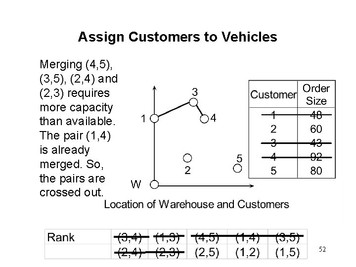
Assign Customers to Vehicles Merging (4, 5), (3, 5), (2, 4) and (2, 3) requires more capacity than available. The pair (1, 4) is already merged. So, the pairs are crossed out. 52

Assign Customers to Vehicles The next pair (2, 5) are merged and assigned to a new vehicle as the capacity available = 200 > 60 + 80 = 140 = capacity required. 53

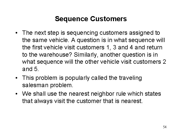
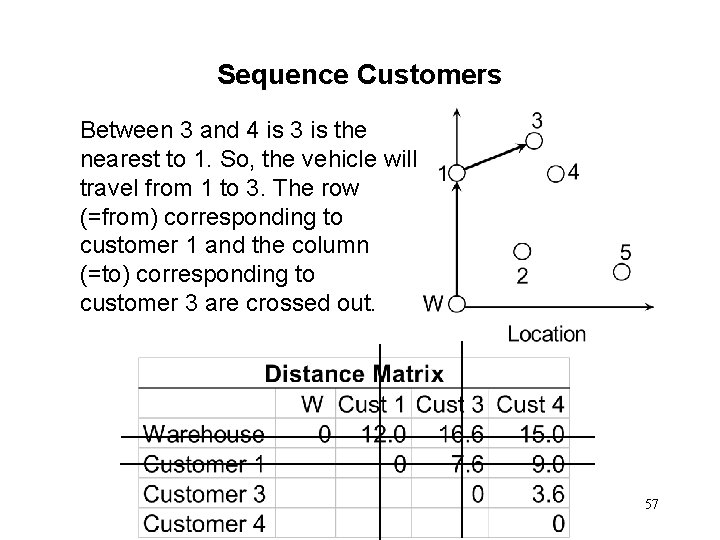
Sequence Customers • The next step is sequencing customers assigned to the same vehicle. A question is in what sequence will the first vehicle visit customers 1, 3 and 4 and return to the warehouse? Similarly, another question is in what sequence will the other vehicle visit customers 2 and 5. • This problem is popularly called the traveling salesman problem. • We shall use the nearest neighbor rule which states that always visit the customer that is nearest. 54

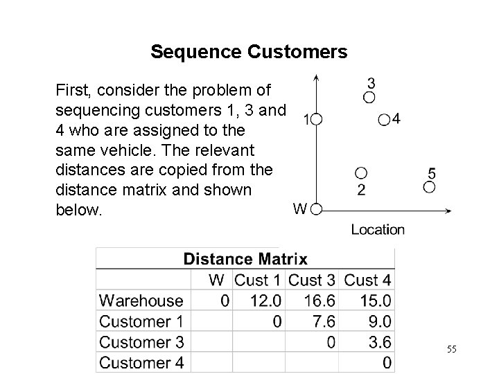
Sequence Customers First, consider the problem of sequencing customers 1, 3 and 4 who are assigned to the same vehicle. The relevant distances are copied from the distance matrix and shown below. 55

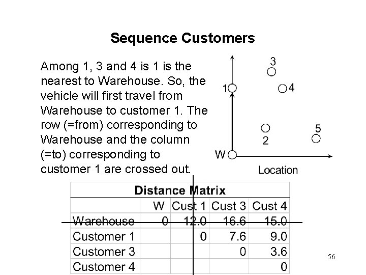
Sequence Customers Among 1, 3 and 4 is 1 is the nearest to Warehouse. So, the vehicle will first travel from Warehouse to customer 1. The row (=from) corresponding to Warehouse and the column (=to) corresponding to customer 1 are crossed out. 56

Sequence Customers Between 3 and 4 is 3 is the nearest to 1. So, the vehicle will travel from 1 to 3. The row (=from) corresponding to customer 1 and the column (=to) corresponding to customer 3 are crossed out. 57

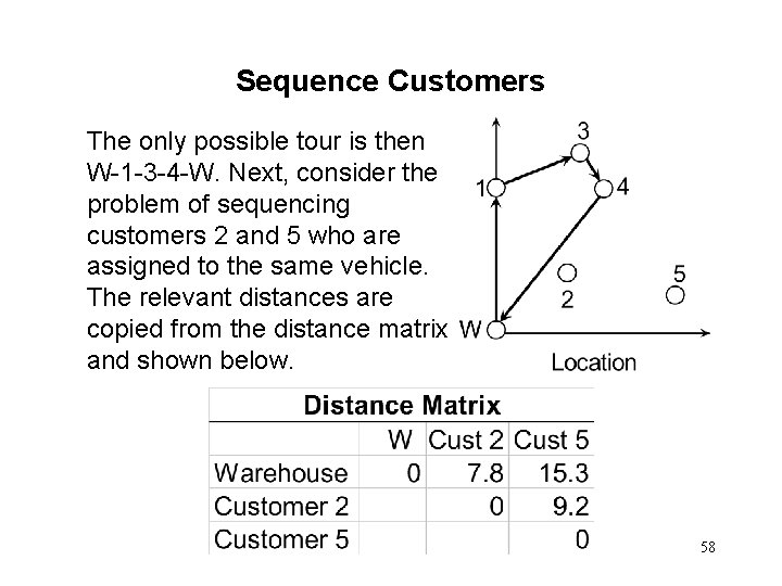
Sequence Customers The only possible tour is then W-1 -3 -4 -W. Next, consider the problem of sequencing customers 2 and 5 who are assigned to the same vehicle. The relevant distances are copied from the distance matrix and shown below. 58

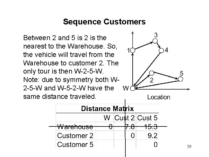
Sequence Customers Between 2 and 5 is 2 is the nearest to the Warehouse. So, the vehicle will travel from the Warehouse to customer 2. The only tour is then W-2 -5 -W. Note: due to symmetry both W 2 -5 -W and W-5 -2 -W have the same distance traveled. 59

Construction and Improvement Procedures • The nearest neighbor rule just discussed is a tour construction procedure which can construct a tour when there is no tour. • The nearest neighbor rule is only a heuristic and does not guarantee optimality. The tour obtained by the heuristic may provide improvement opportunities. • If a tour intersects its own path, the tour can be improved. An improvement procedure will be discussed now. 60

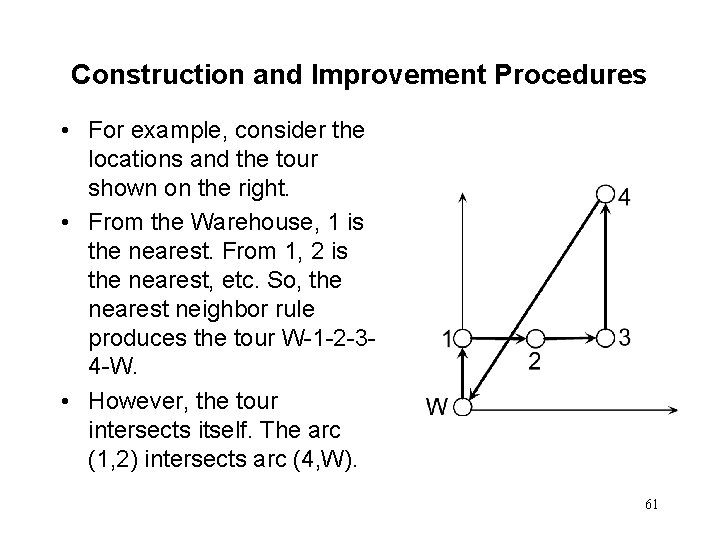
Construction and Improvement Procedures • For example, consider the locations and the tour shown on the right. • From the Warehouse, 1 is the nearest. From 1, 2 is the nearest, etc. So, the nearest neighbor rule produces the tour W-1 -2 -34 -W. • However, the tour intersects itself. The arc (1, 2) intersects arc (4, W). 61

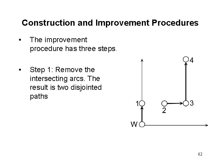
Construction and Improvement Procedures • The improvement procedure has three steps. • Step 1: Remove the intersecting arcs. The result is two disjointed paths 62

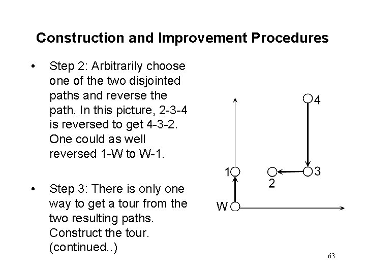
Construction and Improvement Procedures • Step 2: Arbitrarily choose one of the two disjointed paths and reverse the path. In this picture, 2 -3 -4 is reversed to get 4 -3 -2. One could as well reversed 1 -W to W-1. • Step 3: There is only one way to get a tour from the two resulting paths. Construct the tour. (continued. . ) 63

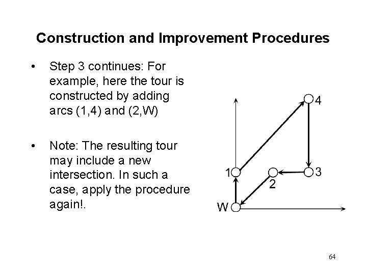
Construction and Improvement Procedures • Step 3 continues: For example, here the tour is constructed by adding arcs (1, 4) and (2, W) • Note: The resulting tour may include a new intersection. In such a case, apply the procedure again!. 64

READING AND EXERCISES Lesson 7 Reading: – Section 6. 6 pp. 325 -330 (4 th Ed. ), pp. 315 -320 (5 th Ed. ) Exercises: – 6. 16 p. 331 (4 th Ed. ), p. 321 (5 th Ed. ) 65