Supplement E Simulation Copyright 2013 Pearson Education Inc

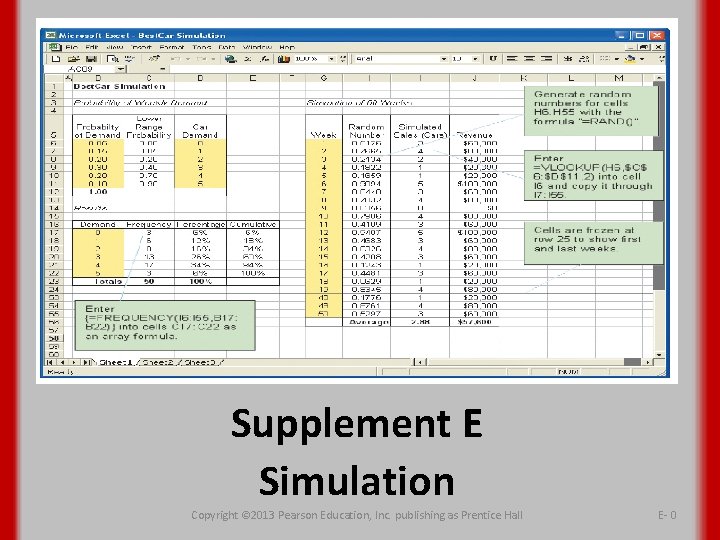
Supplement E Simulation Copyright © 2013 Pearson Education, Inc. publishing as Prentice Hall E- 0

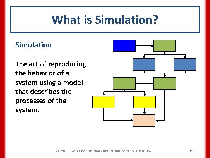
What is Simulation? Simulation The act of reproducing the behavior of a system using a model that describes the processes of the system. Copyright © 2013 Pearson Education, Inc. publishing as Prentice Hall E- 02

Reasons for Using Simulation • To analyze a problem when the relationship between variables is nonlinear, or when the situation involves too many variables or constraints to handle with optimizing approaches. • To conduct experiments without disrupting real systems. • To obtain operating characteristic estimates in much less time (time compression). • To sharpen managerial decision-making skills through gaming. Copyright © 2013 Pearson Education, Inc. publishing as Prentice Hall E -03

The Simulation Process • Monte Carlo simulation – A simulation process that uses random numbers to generate simulation events • Data collection • Random-number assignment – A random number is a number that has the same probability of being selected as any other number (see Appendix 2) • Model formulation Copyright © 2013 Pearson Education, Inc. publishing as Prentice Hall E - 04

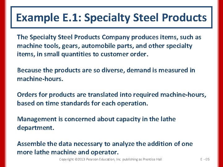
Example E. 1: Specialty Steel Products The Specialty Steel Products Company produces items, such as machine tools, gears, automobile parts, and other specialty items, in small quantities to customer order. Because the products are so diverse, demand is measured in machine-hours. Orders for products are translated into required machine-hours, based on time standards for each operation. Management is concerned about capacity in the lathe department. Assemble the data necessary to analyze the addition of one more lathe machine and operator. Copyright © 2013 Pearson Education, Inc. publishing as Prentice Hall E - 05

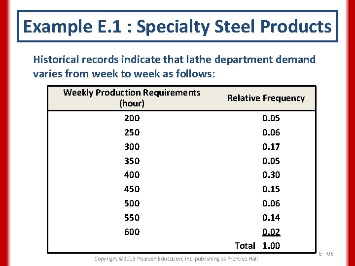
Example E. 1 : Specialty Steel Products Historical records indicate that lathe department demand varies from week to week as follows: Weekly Production Requirements (hour) 200 250 300 350 400 450 500 550 600 Relative Frequency 0. 05 0. 06 0. 17 0. 05 0. 30 0. 15 0. 06 0. 14 0. 02 Total 1. 00 Copyright © 2013 Pearson Education, Inc. publishing as Prentice Hall E - 06

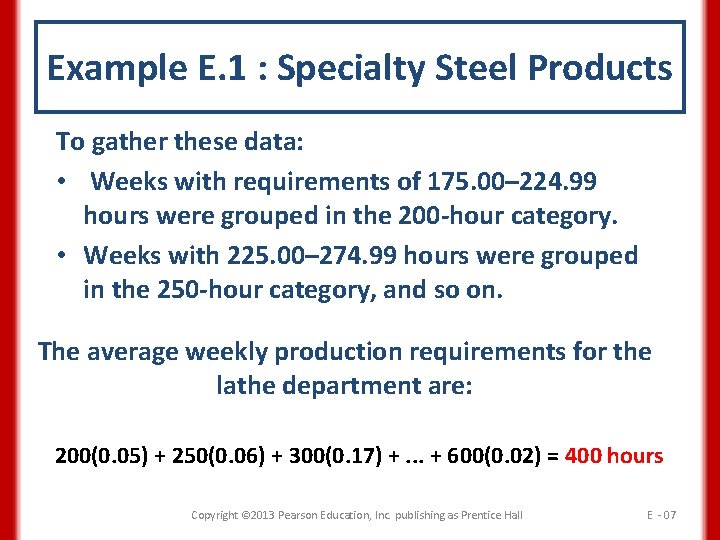
Example E. 1 : Specialty Steel Products To gather these data: • Weeks with requirements of 175. 00– 224. 99 hours were grouped in the 200 -hour category. • Weeks with 225. 00– 274. 99 hours were grouped in the 250 -hour category, and so on. The average weekly production requirements for the lathe department are: 200(0. 05) + 250(0. 06) + 300(0. 17) +. . . + 600(0. 02) = 400 hours Copyright © 2013 Pearson Education, Inc. publishing as Prentice Hall E - 07

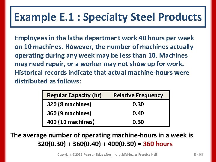
Example E. 1 : Specialty Steel Products Employees in the lathe department work 40 hours per week on 10 machines. However, the number of machines actually operating during any week may be less than 10. Machines may need repair, or a worker may not show up for work. Historical records indicate that actual machine-hours were distributed as follows: Regular Capacity (hr) 320 (8 machines) 360 (9 machines) 400 (10 machines) Relative Frequency 0. 30 0. 40 0. 30 The average number of operating machine-hours in a week is 320(0. 30) + 360(0. 40) + 400(0. 30) = 360 hours Copyright © 2013 Pearson Education, Inc. publishing as Prentice Hall E - 08

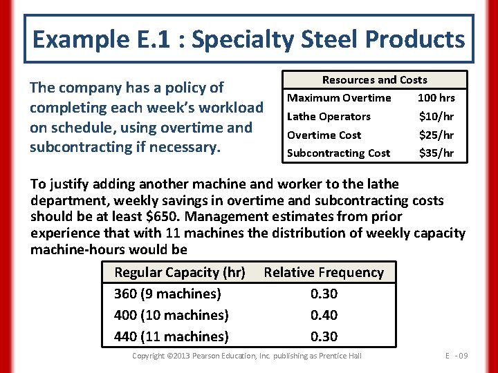
Example E. 1 : Specialty Steel Products The company has a policy of completing each week’s workload on schedule, using overtime and subcontracting if necessary. Resources and Costs Maximum Overtime 100 hrs Lathe Operators $10/hr Overtime Cost $25/hr Subcontracting Cost $35/hr To justify adding another machine and worker to the lathe department, weekly savings in overtime and subcontracting costs should be at least $650. Management estimates from prior experience that with 11 machines the distribution of weekly capacity machine-hours would be Regular Capacity (hr) Relative Frequency 360 (9 machines) 0. 30 400 (10 machines) 0. 40 440 (11 machines) 0. 30 Copyright © 2013 Pearson Education, Inc. publishing as Prentice Hall E - 09

Random-Number Assignment • Random number – A number that has the same probability of being selected as any other number • Events in a simulation can be generated in an unbiased way if random numbers are assigned to the events in the same proportion as their probability of occurrence. Copyright © 2013 Pearson Education, Inc. publishing as Prentice Hall E - 10

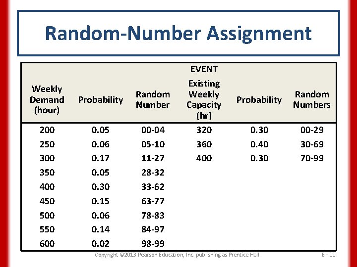
Random-Number Assignment Weekly Demand (hour) Probability Random Number 200 250 300 350 400 450 500 550 600 0. 05 0. 06 0. 17 0. 05 0. 30 0. 15 0. 06 0. 14 0. 02 00 -04 05 -10 11 -27 28 -32 33 -62 63 -77 78 -83 84 -97 98 -99 EVENT Existing Weekly Capacity (hr) 320 360 400 Probability Random Numbers 0. 30 0. 40 0. 30 00 -29 30 -69 70 -99 Copyright © 2013 Pearson Education, Inc. publishing as Prentice Hall E - 11

Model Formulation • Decision variables • Uncontrollable variables (random) • Dependent variables Copyright © 2013 Pearson Education, Inc. publishing as Prentice Hall E - 12

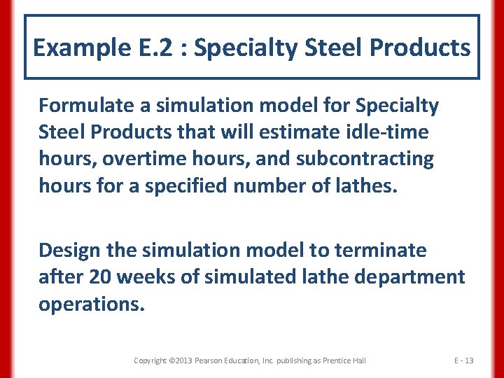
Example E. 2 : Specialty Steel Products Formulate a simulation model for Specialty Steel Products that will estimate idle-time hours, overtime hours, and subcontracting hours for a specified number of lathes. Design the simulation model to terminate after 20 weeks of simulated lathe department operations. Copyright © 2013 Pearson Education, Inc. publishing as Prentice Hall E - 13

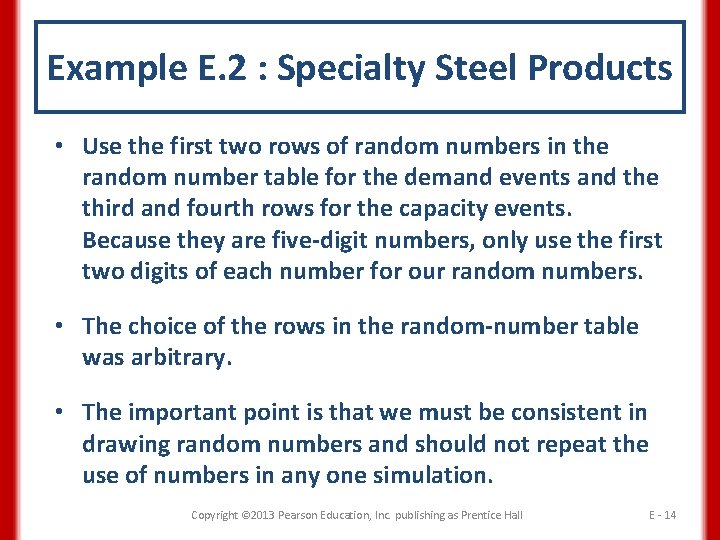
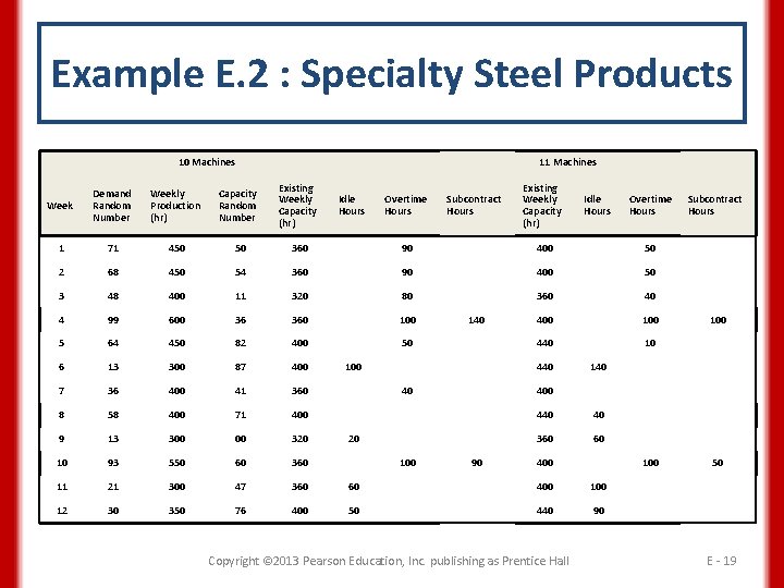
Example E. 2 : Specialty Steel Products • Use the first two rows of random numbers in the random number table for the demand events and the third and fourth rows for the capacity events. Because they are five-digit numbers, only use the first two digits of each number for our random numbers. • The choice of the rows in the random-number table was arbitrary. • The important point is that we must be consistent in drawing random numbers and should not repeat the use of numbers in any one simulation. Copyright © 2013 Pearson Education, Inc. publishing as Prentice Hall E - 14

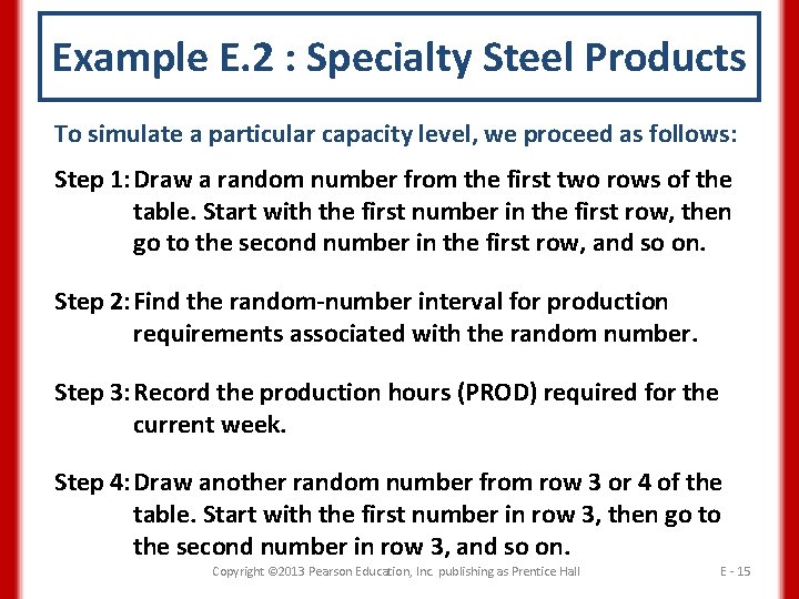
Example E. 2 : Specialty Steel Products To simulate a particular capacity level, we proceed as follows: Step 1: Draw a random number from the first two rows of the table. Start with the first number in the first row, then go to the second number in the first row, and so on. Step 2: Find the random-number interval for production requirements associated with the random number. Step 3: Record the production hours (PROD) required for the current week. Step 4: Draw another random number from row 3 or 4 of the table. Start with the first number in row 3, then go to the second number in row 3, and so on. Copyright © 2013 Pearson Education, Inc. publishing as Prentice Hall E - 15

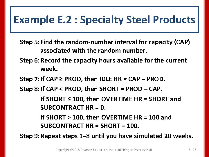
Example E. 2 : Specialty Steel Products Step 5: Find the random-number interval for capacity (CAP) associated with the random number. Step 6: Record the capacity hours available for the current week. Step 7: If CAP ≥ PROD, then IDLE HR = CAP – PROD. Step 8: If CAP < PROD, then SHORT = PROD – CAP. If SHORT ≤ 100, then OVERTIME HR = SHORT and SUBCONTRACT HR = 0. If SHORT > 100, then OVERTIME HR = 100 and SUBCONTRACT HR = SHORT – 100. Step 9: Repeat steps 1– 8 until you have simulated 20 weeks. Copyright © 2013 Pearson Education, Inc. publishing as Prentice Hall E - 16

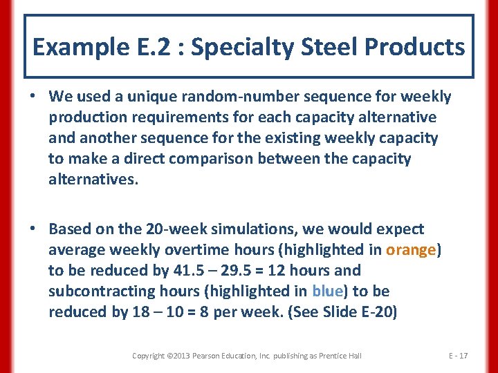
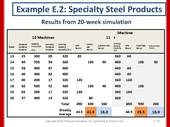
Example E. 2 : Specialty Steel Products • We used a unique random-number sequence for weekly production requirements for each capacity alternative and another sequence for the existing weekly capacity to make a direct comparison between the capacity alternatives. • Based on the 20 -week simulations, we would expect average weekly overtime hours (highlighted in orange) to be reduced by 41. 5 – 29. 5 = 12 hours and subcontracting hours (highlighted in blue) to be reduced by 18 – 10 = 8 per week. (See Slide E-20) Copyright © 2013 Pearson Education, Inc. publishing as Prentice Hall E - 17

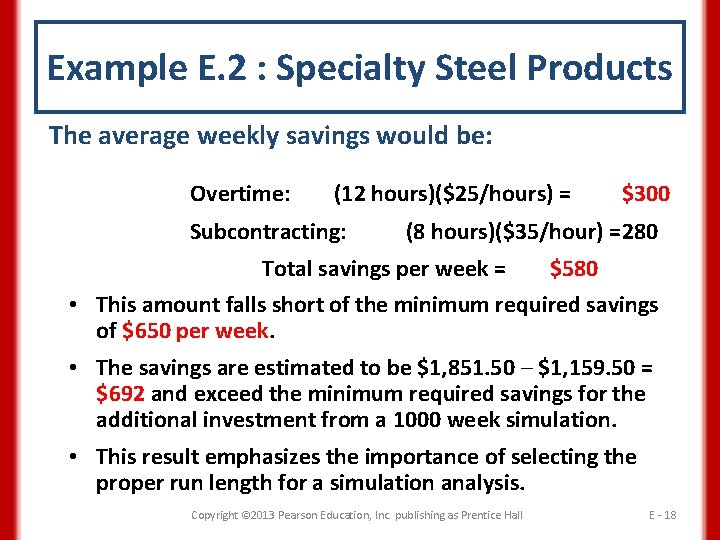
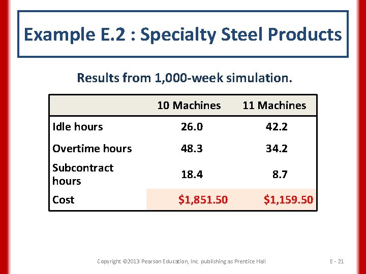
Example E. 2 : Specialty Steel Products The average weekly savings would be: Overtime: (12 hours)($25/hours) = Subcontracting: $300 (8 hours)($35/hour) =280 Total savings per week = $580 • This amount falls short of the minimum required savings of $650 per week. • The savings are estimated to be $1, 851. 50 – $1, 159. 50 = $692 and exceed the minimum required savings for the additional investment from a 1000 week simulation. • This result emphasizes the importance of selecting the proper run length for a simulation analysis. Copyright © 2013 Pearson Education, Inc. publishing as Prentice Hall E - 18

Example E. 2 : Specialty Steel Products 10 Machines 11 Machines Week Demand Random Number Weekly Production (hr) Capacity Random Number Existing Weekly Capacity (hr) 1 71 450 50 360 90 400 50 2 68 450 54 360 90 400 50 3 48 400 11 320 80 360 40 4 99 600 36 360 100 400 100 5 64 450 82 400 50 440 10 6 13 300 87 400 7 36 400 41 360 8 58 400 71 400 9 13 300 00 320 10 93 550 60 360 11 21 300 47 360 60 400 12 30 350 76 400 50 440 90 Idle Hours Overtime Hours Subcontract Hours 140 100 Existing Weekly Capacity (hr) 440 40 Overtime Hours Subcontract Hours 100 140 400 20 100 Idle Hours 90 440 40 360 60 400 Copyright © 2013 Pearson Education, Inc. publishing as Prentice Hall 100 50 E - 19

Example E. 2: Specialty Steel Products Results from 20 -week simulation 11 s 10 Machines Week Demand Random Number Weekly Production (hr) Capacity Random Number Existing Weekly Capacity (hr) Idle Hours Overti me Hours Subcontract Hours 20 Machine Existing Weekly Capacity (hr) Idle Hours 360 60 13 23 300 09 320 14 89 550 54 360 15 58 400 87 400 440 40 16 46 400 82 400 440 40 17 00 200 17 320 360 18 82 500 52 360 19 02 200 17 320 20 37 400 19 320 100 90 120 100 40 120 400 80 100 400 360 Overtime Hours Subcontract Hours 50 100 160 360 Total 490 830 360 890 590 200 Weekly average 24. 5 41. 5 18. 0 44. 5 29. 5 10. 0 Copyright © 2013 Pearson Education, Inc. publishing as Prentice Hall E- 20

Example E. 2 : Specialty Steel Products Results from 1, 000 -week simulation. 10 Machines 11 Machines Idle hours 26. 0 42. 2 Overtime hours 48. 3 34. 2 Subcontract hours 18. 4 8. 7 Cost $1, 851. 50 $1, 159. 50 Copyright © 2013 Pearson Education, Inc. publishing as Prentice Hall E - 21

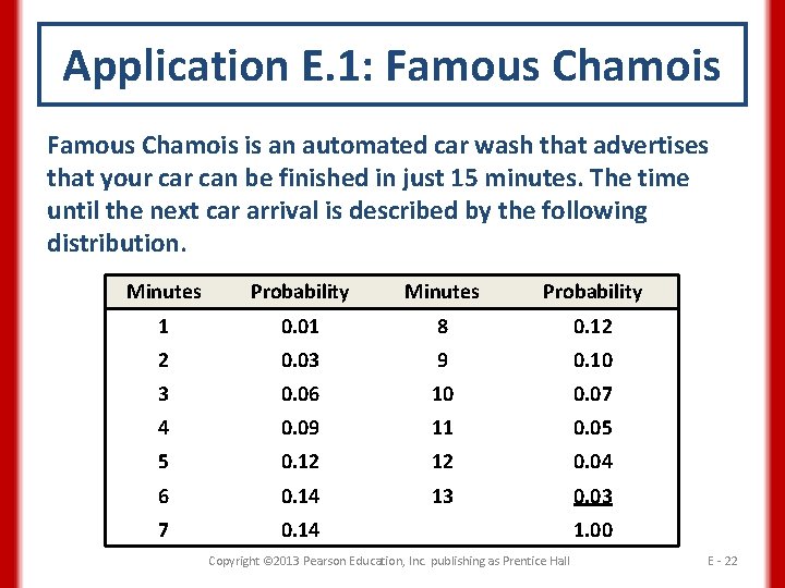
Application E. 1: Famous Chamois is an automated car wash that advertises that your can be finished in just 15 minutes. The time until the next car arrival is described by the following distribution. Minutes Probability 1 0. 01 8 0. 12 2 0. 03 9 0. 10 3 0. 06 10 0. 07 4 0. 09 11 0. 05 5 0. 12 12 0. 04 6 0. 14 13 0. 03 7 0. 14 Copyright © 2013 Pearson Education, Inc. publishing as Prentice Hall 1. 00 E - 22

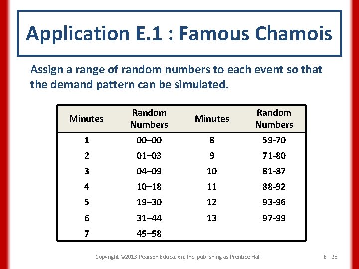
Application E. 1 : Famous Chamois Assign a range of random numbers to each event so that the demand pattern can be simulated. Minutes Random Numbers 1 00– 00 8 59 -70 2 01– 03 9 71 -80 3 04– 09 10 81 -87 4 10– 18 11 88 -92 5 19– 30 12 93 -96 6 31– 44 13 97 -99 7 45– 58 Copyright © 2013 Pearson Education, Inc. publishing as Prentice Hall E - 23

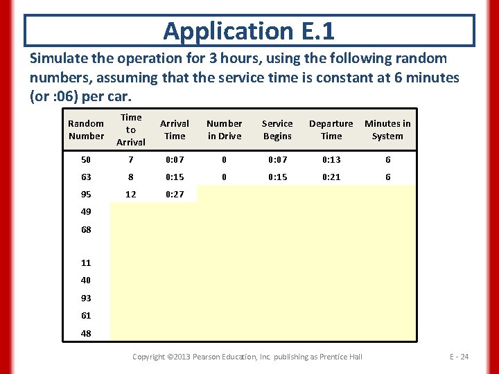
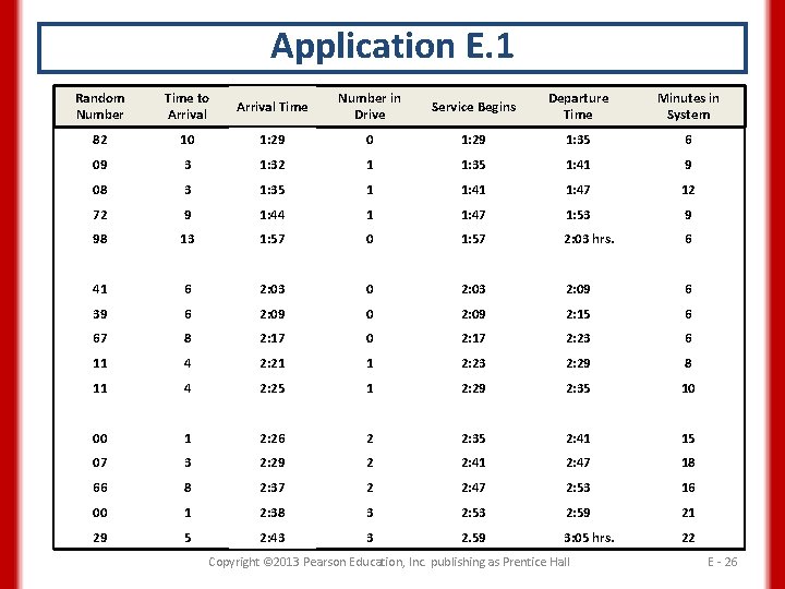
Application E. 1 Simulate the operation for 3 hours, using the following random numbers, assuming that the service time is constant at 6 minutes (or : 06) per car. Random Number Time to Arrival Time Number in Drive Service Begins Departure Time Minutes in System 50 7 0: 07 0: 13 6 63 8 0: 15 0: 21 6 95 12 0: 27 49 68 11 40 93 61 48 Copyright © 2013 Pearson Education, Inc. publishing as Prentice Hall E - 24

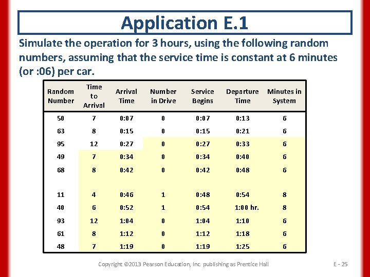
Application E. 1 Simulate the operation for 3 hours, using the following random numbers, assuming that the service time is constant at 6 minutes (or : 06) per car. Random Number Time to Arrival Time Number in Drive Service Begins Departure Time Minutes in System 50 7 0: 07 0: 13 6 63 8 0: 15 0: 21 6 95 12 0: 27 0: 33 6 49 7 0: 34 0: 40 6 68 8 0: 42 0: 48 6 11 4 0: 46 1 0: 48 0: 54 8 40 6 0: 52 1 0: 54 1: 00 hr. 8 93 12 1: 04 0 1: 04 1: 10 6 61 8 1: 12 0 1: 12 1: 18 6 48 7 1: 19 0 1: 19 1: 25 6 Copyright © 2013 Pearson Education, Inc. publishing as Prentice Hall E - 25

Application E. 1 Random Number Time to Arrival Time Number in Drive Service Begins Departure Time Minutes in System 82 10 1: 29 1: 35 6 09 3 1: 32 1 1: 35 1: 41 9 08 3 1: 35 1 1: 47 12 72 9 1: 44 1 1: 47 1: 53 9 98 13 1: 57 0 1: 57 2: 03 hrs. 6 41 6 2: 03 0 2: 03 2: 09 6 39 6 2: 09 0 2: 09 2: 15 6 67 8 2: 17 0 2: 17 2: 23 6 11 4 2: 21 1 2: 23 2: 29 8 11 4 2: 25 1 2: 29 2: 35 10 00 1 2: 26 2 2: 35 2: 41 15 07 3 2: 29 2 2: 41 2: 47 18 66 8 2: 37 2 2: 47 2: 53 16 00 1 2: 38 3 2: 59 21 29 5 2: 43 3 2. 59 3: 05 hrs. 22 Copyright © 2013 Pearson Education, Inc. publishing as Prentice Hall E - 26

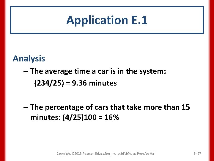
Application E. 1 Analysis – The average time a car is in the system: (234/25) = 9. 36 minutes – The percentage of cars that take more than 15 minutes: (4/25)100 = 16% Copyright © 2013 Pearson Education, Inc. publishing as Prentice Hall E- 27

Computer Simulation • Steady state – The state that occurs when the simulation is repeated over enough time that the average results for performance measures remain constant. • Manual simulations can be excessively timeconsuming. • Simple simulation models can be developed using Excel. Copyright © 2013 Pearson Education, Inc. publishing as Prentice Hall E - 28

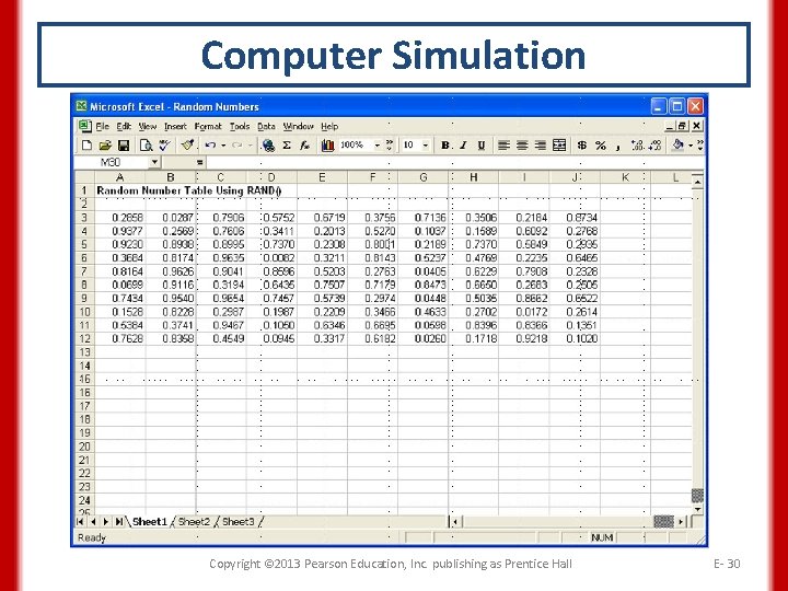
Computer Simulation • Random numbers can be generated using the RAND function. • Excel can translate random numbers into values for the uncontrollable variables using the VLOOKUP function. Copyright © 2013 Pearson Education, Inc. publishing as Prentice Hall E - 29

Computer Simulation Copyright © 2013 Pearson Education, Inc. publishing as Prentice Hall E- 30

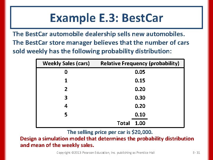
Example E. 3: Best. Car The Best. Car automobile dealership sells new automobiles. The Best. Car store manager believes that the number of cars sold weekly has the following probability distribution: Weekly Sales (cars) 0 1 2 3 4 5 Relative Frequency (probability) 0. 05 0. 15 0. 20 0. 30 0. 20 0. 10 Total 1. 00 The selling price per car is $20, 000. Design a simulation model that determines the probability distribution and mean of the weekly sales. Copyright © 2013 Pearson Education, Inc. publishing as Prentice Hall E- 31

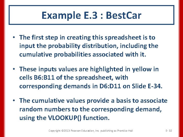
Example E. 3 : Best. Car • The first step in creating this spreadsheet is to input the probability distribution, including the cumulative probabilities associated with it. • These inputs values are highlighted in yellow in cells B 6: B 11 of the spreadsheet, with corresponding demands in D 6: D 11 on Slide E-34. • The cumulative values provide a basis to associate random numbers to the corresponding demand, using the VLOOKUP() function. Copyright © 2013 Pearson Education, Inc. publishing as Prentice Hall E- 32

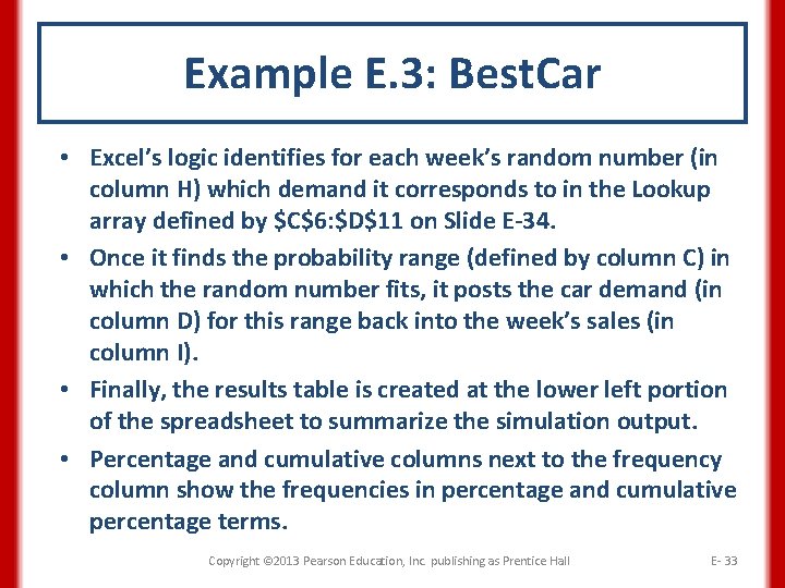
Example E. 3: Best. Car • Excel’s logic identifies for each week’s random number (in column H) which demand it corresponds to in the Lookup array defined by $C$6: $D$11 on Slide E-34. • Once it finds the probability range (defined by column C) in which the random number fits, it posts the car demand (in column D) for this range back into the week’s sales (in column I). • Finally, the results table is created at the lower left portion of the spreadsheet to summarize the simulation output. • Percentage and cumulative columns next to the frequency column show the frequencies in percentage and cumulative percentage terms. Copyright © 2013 Pearson Education, Inc. publishing as Prentice Hall E- 33

Example E. 3 : Best. Car Copyright © 2013 Pearson Education, Inc. publishing as Prentice Hall E - 34

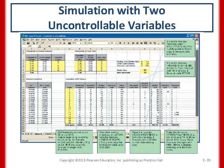
Simulation with Two Uncontrollable Variables Copyright © 2013 Pearson Education, Inc. publishing as Prentice Hall E- 35

Simulation with More Advanced Software • Even more computer power comes from commercial, prewritten simulation software. • Simulation programming can be done in generalpurpose programming languages such as VISUAL BASIC, FORTRAN, or C++. • Special simulation languages, such as GPSS, SIMSCRIPT, and SLAM, are also available. • Simulation is also possible with powerful PC-based packages, such as Sim. Quick, Extend, SIMPROCESS, Pro. Model, and Witness. Copyright © 2013 Pearson Education, Inc. publishing as Prentice Hall E- 36

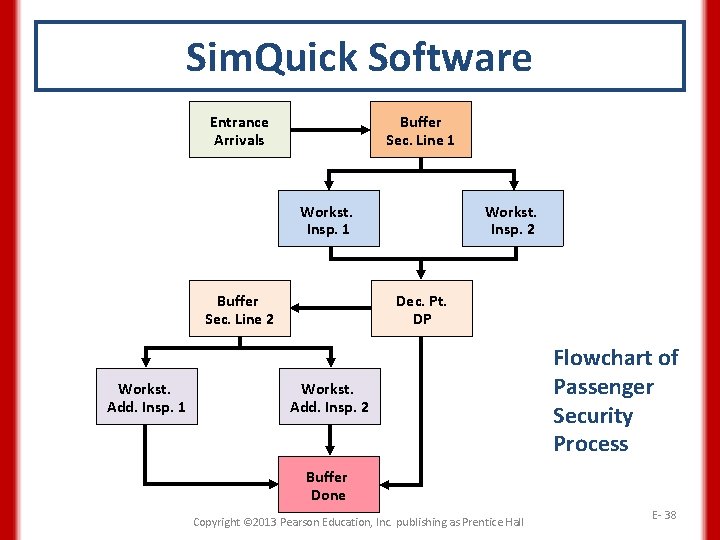
Sim. Quick Software • Easy-to-use package that is simply an Excel spreadsheet with some macros. • Models can be created for a variety of simple processes. • A first step with Sim. Quick is to draw a flowchart of the process using Sim. Quick’s building blocks. • Information describing each building block is entered into Sim. Quick tables. Copyright © 2013 Pearson Education, Inc. publishing as Prentice Hall E- 37

Sim. Quick Software Entrance Arrivals Buffer Sec. Line 1 Workst. Insp. 1 Buffer Sec. Line 2 Workst. Add. Insp. 1 Workst. Insp. 2 Dec. Pt. DP Workst. Add. Insp. 2 Flowchart of Passenger Security Process Buffer Done Copyright © 2013 Pearson Education, Inc. publishing as Prentice Hall E- 38

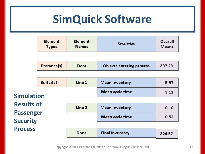
Sim. Quick Software Element Types Element Names Statistics Overall Means Entrance(s) Door Objects entering process 237. 23 Buffer(s) Line 1 Simulation Results of Passenger Security Process Line 2 Done Mean Inventory 5. 97 Mean cycle time 3. 12 Mean Inventory 0. 10 Mean cycle time 0. 53 Final Inventory Copyright © 2013 Pearson Education, Inc. publishing as Prentice Hall 224. 57 E- 39

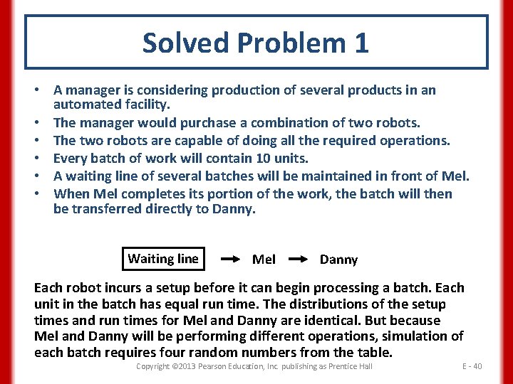
Solved Problem 1 • A manager is considering production of several products in an automated facility. • The manager would purchase a combination of two robots. • The two robots are capable of doing all the required operations. • Every batch of work will contain 10 units. • A waiting line of several batches will be maintained in front of Mel. • When Mel completes its portion of the work, the batch will then be transferred directly to Danny. Waiting line Mel Danny Each robot incurs a setup before it can begin processing a batch. Each unit in the batch has equal run time. The distributions of the setup times and run times for Mel and Danny are identical. But because Mel and Danny will be performing different operations, simulation of each batch requires four random numbers from the table. Copyright © 2013 Pearson Education, Inc. publishing as Prentice Hall E - 40

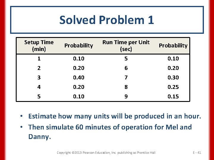
Solved Problem 1 Setup Time (min) Probability Run Time per Unit (sec) Probability 1 0. 10 5 0. 10 2 0. 20 6 0. 20 3 0. 40 7 0. 30 4 0. 20 8 0. 25 5 0. 10 9 0. 15 • Estimate how many units will be produced in an hour. • Then simulate 60 minutes of operation for Mel and Danny. Copyright © 2013 Pearson Education, Inc. publishing as Prentice Hall E - 41

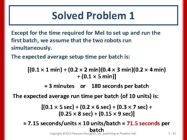
Solved Problem 1 Except for the time required for Mel to set up and run the first batch, we assume that the two robots run simultaneously. The expected average setup time per batch is: [(0. 1 1 min) + (0. 2 2 min)(0. 4 3 min)(0. 2 4 min) + (0. 1 5 min)] = 3 minutes or 180 seconds per batch The expected average run time per batch (of 10 units) is: [(0. 1 5 sec) + (0. 2 6 sec) + (0. 3 7 sec) + (0. 25 8 sec) + (0. 15 9 sec)] = 7. 15 seconds/units 10 units/batch = 71. 5 seconds per batch Copyright © 2013 Pearson Education, Inc. publishing as Prentice Hall E - 42

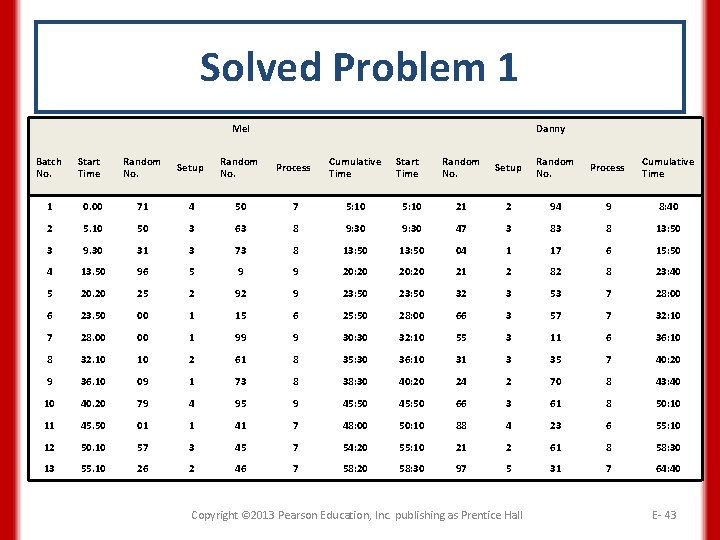
Solved Problem 1 Mel Batch No. Start Time Danny Random No. Setup Random No. Process Cumulative Time Start Time Random No. Setup Random No. Process Cumulative Time 1 0. 00 71 4 50 7 5: 10 21 2 94 9 8: 40 2 5. 10 50 3 63 8 9: 30 47 3 83 8 13: 50 3 9. 30 31 3 73 8 13: 50 04 1 17 6 15: 50 4 13. 50 96 5 9 9 20: 20 21 2 82 8 23: 40 5 20. 20 25 2 92 9 23: 50 32 3 53 7 28: 00 6 23. 50 00 1 15 6 25: 50 28: 00 66 3 57 7 32: 10 7 28. 00 00 1 99 9 30: 30 32: 10 55 3 11 6 36: 10 8 32. 10 10 2 61 8 35: 30 36: 10 31 3 35 7 40: 20 9 36. 10 09 1 73 8 38: 30 40: 20 24 2 70 8 43: 40 10 40. 20 79 4 95 9 45: 50 66 3 61 8 50: 10 11 45. 50 01 1 41 7 48: 00 50: 10 88 4 23 6 55: 10 12 50. 10 57 3 45 7 54: 20 55: 10 21 2 61 8 58: 30 13 55. 10 26 2 46 7 58: 20 58: 30 97 5 31 7 64: 40 Copyright © 2013 Pearson Education, Inc. publishing as Prentice Hall E- 43

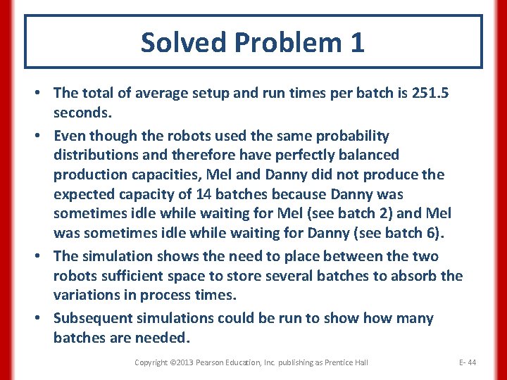
Solved Problem 1 • The total of average setup and run times per batch is 251. 5 seconds. • Even though the robots used the same probability distributions and therefore have perfectly balanced production capacities, Mel and Danny did not produce the expected capacity of 14 batches because Danny was sometimes idle while waiting for Mel (see batch 2) and Mel was sometimes idle while waiting for Danny (see batch 6). • The simulation shows the need to place between the two robots sufficient space to store several batches to absorb the variations in process times. • Subsequent simulations could be run to show many batches are needed. Copyright © 2013 Pearson Education, Inc. publishing as Prentice Hall E- 44

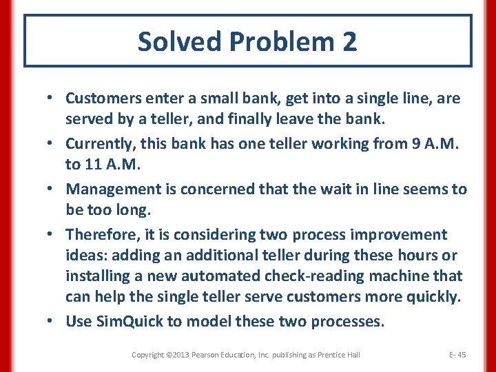
Solved Problem 2 • Customers enter a small bank, get into a single line, are served by a teller, and finally leave the bank. • Currently, this bank has one teller working from 9 A. M. to 11 A. M. • Management is concerned that the wait in line seems to be too long. • Therefore, it is considering two process improvement ideas: adding an additional teller during these hours or installing a new automated check-reading machine that can help the single teller serve customers more quickly. • Use Sim. Quick to model these two processes. Copyright © 2013 Pearson Education, Inc. publishing as Prentice Hall E- 45

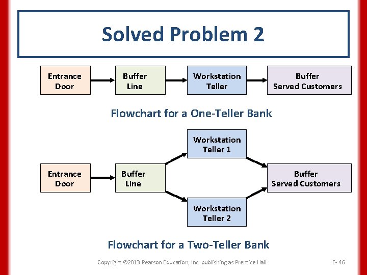
Solved Problem 2 Entrance Door Buffer Line Workstation Teller Buffer Served. Customers Flowchart for a One-Teller Bank Workstation Teller 1 1 Teller Entrance Door Buffer Line Buffer Served. Customers Workstation Teller 2 2 Teller Flowchart for a Two-Teller Bank Copyright © 2013 Pearson Education, Inc. publishing as Prentice Hall E- 46

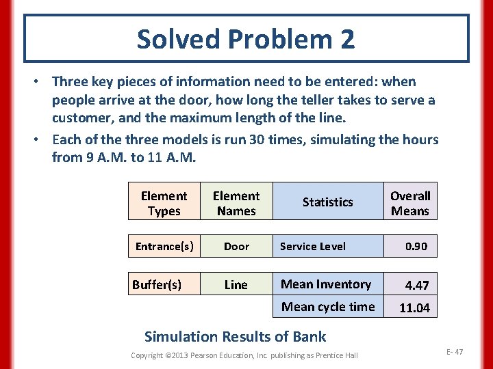
Solved Problem 2 • Three key pieces of information need to be entered: when people arrive at the door, how long the teller takes to serve a customer, and the maximum length of the line. • Each of the three models is run 30 times, simulating the hours from 9 A. M. to 11 A. M. Element Types Element Names Entrance(s) Door Service Level 0. 90 Buffer(s) Line Mean Inventory 4. 47 Mean cycle time 11. 04 Statistics Overall Means Simulation Results of Bank Copyright © 2013 Pearson Education, Inc. publishing as Prentice Hall E- 47

Solved Problem 2 • The numbers shown are averages across the 30 simulations. • The service level for Door tells us that 90 percent of the simulated customers who arrived at the bank were able to get into Line. • The mean inventory for Line tells us that 4. 47 simulated customers were standing in line. • The mean cycle time tells us that simulated customers waited an average of 11. 04 minutes in line. • When we run the model with two tellers, we find that the service level increases to 100 percent, the mean inventory in Line decreases to 0. 37 customer, and the mean cycle time drops to 0. 71 minute. • When we run the one-teller model with the faster check-reading machine we find that the service level is 97 percent, the mean inventory in Line is 2. 89 customers, and the mean cycle time is 6. 21 minutes. E- 48 Copyright © 2013 Pearson Education, Inc. publishing as Prentice Hall

All rights reserved. No part of this publication may be reproduced, stored in a retrieval system, or transmitted, in any form or by any means, electronic, mechanical, photocopying, recording, or otherwise, without the prior written permission of the publisher. Printed in the United States of America. Copyright © 2013 Pearson Education, Inc. publishing as Prentice Hall E- 49