StateSpace Models DNT 354 CONTROL PRINCIPLE Date 29072015

State-Space Models DNT 354 – CONTROL PRINCIPLE Date: 29/07/2015 Prepared by: Nor Shaifudin Bin Abdul Hamid Email: norshaifudin@unimap. edu. my

CONTENTS • Introduction • State-Space Model • Signal Flow Graph

INTRODUCTION • The basic questions that will be addressed in state-space approach include: i. What are state-space models? ii. Why should we use them? iii. How are they related to the transfer function used in classical control system? iv. How do we develop a space-state model?

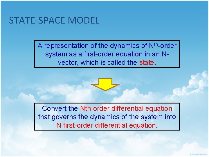
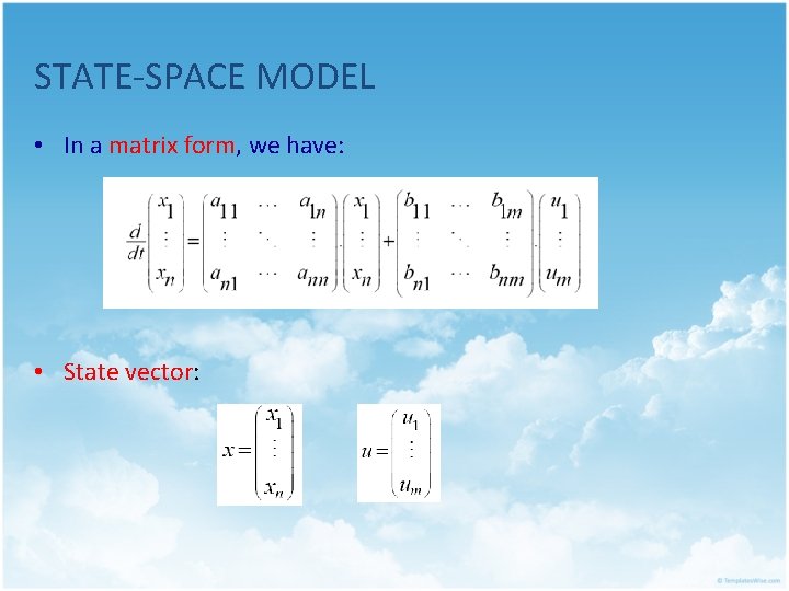
STATE-SPACE MODEL A representation of the dynamics of Nth-order system as a first-order equation in an Nvector, which is called the state. Convert the Nth-order differential equation that governs the dynamics of the system into N first-order differential equation.

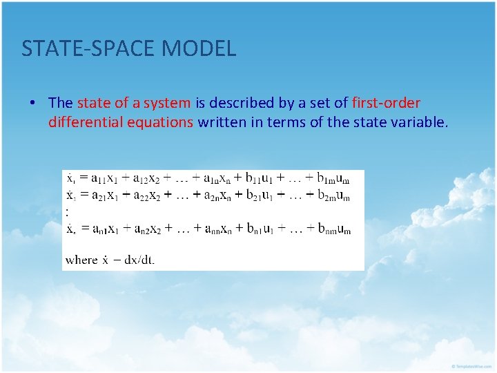
STATE-SPACE MODEL • The state of a system is described by a set of first-order differential equations written in terms of the state variable.

STATE-SPACE MODEL • In a matrix form, we have: • State vector:

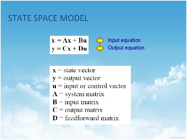
STATE SPACE MODEL Input equation Output equation

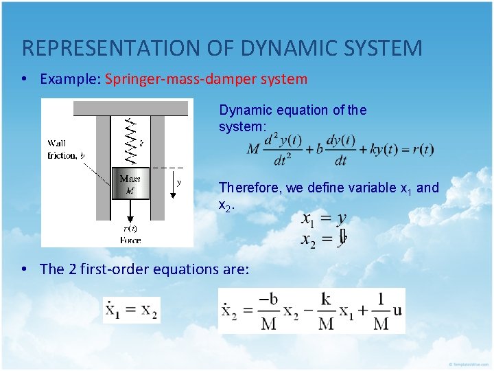
REPRESENTATION OF DYNAMIC SYSTEM • Example: Springer-mass-damper system Dynamic equation of the system: Therefore, we define variable x 1 and x 2. • The 2 first-order equations are:

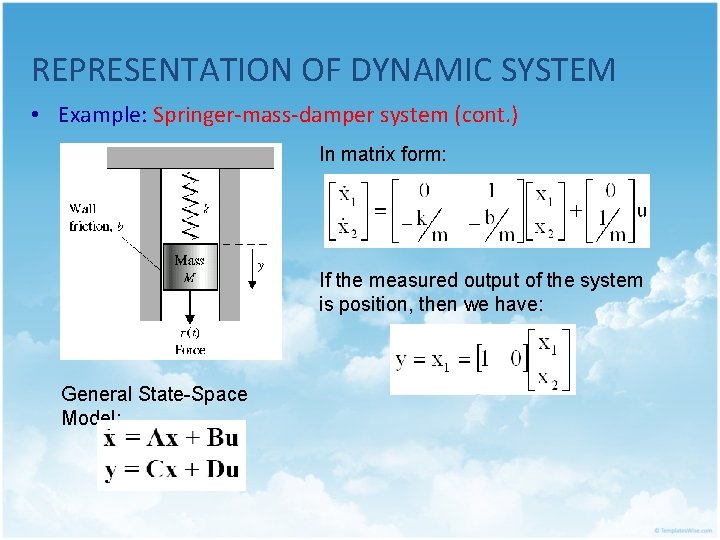
REPRESENTATION OF DYNAMIC SYSTEM • Example: Springer-mass-damper system (cont. ) In matrix form: If the measured output of the system is position, then we have: General State-Space Model:

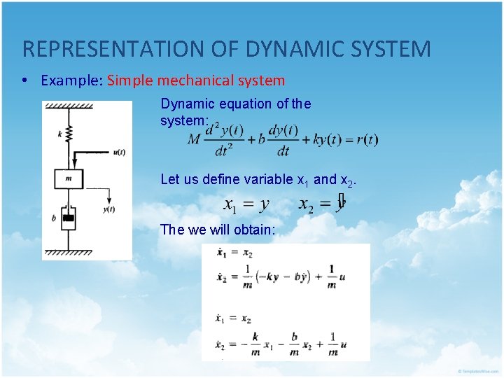
REPRESENTATION OF DYNAMIC SYSTEM • Example: Simple mechanical system Dynamic equation of the system: Let us define variable x 1 and x 2. The we will obtain:

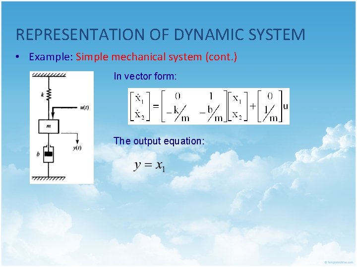
REPRESENTATION OF DYNAMIC SYSTEM • Example: Simple mechanical system (cont. ) In vector form: The output equation:

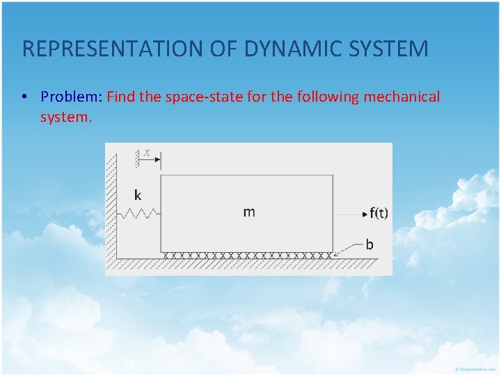
REPRESENTATION OF DYNAMIC SYSTEM • Problem: Find the space-state for the following mechanical system.

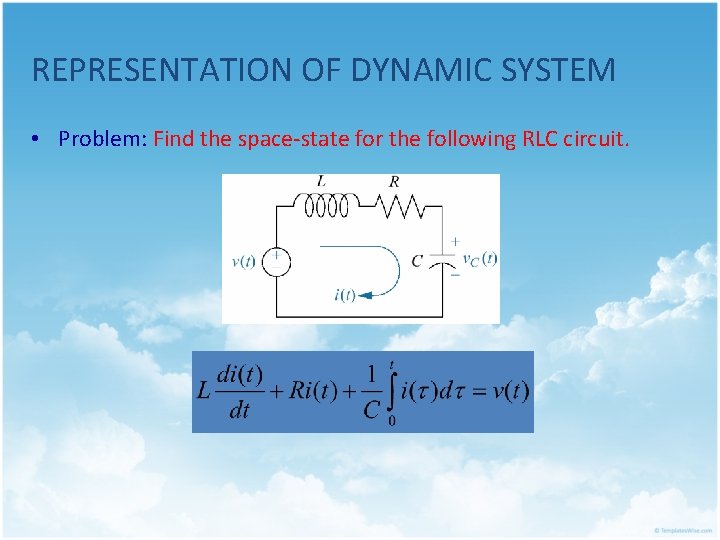
REPRESENTATION OF DYNAMIC SYSTEM • Problem: Find the space-state for the following RLC circuit.

SIGNAL FLOW GRAPH • A signal flow graph is a graphical representation of the relationships between the variables of a set of linear algebraic equations. • The basic element of a signal flow graph is a unidirectional path segments called branch. • The input and output points or junctions are called nodes. • A path is a branch or continuous sequence or branches that can be traversed from one signal node to another signal node. • A loop is a closed path that originates and terminates on the same node, and along the path no node is met twice. • Two loops are said to be non-touching if they do not have a same common node.

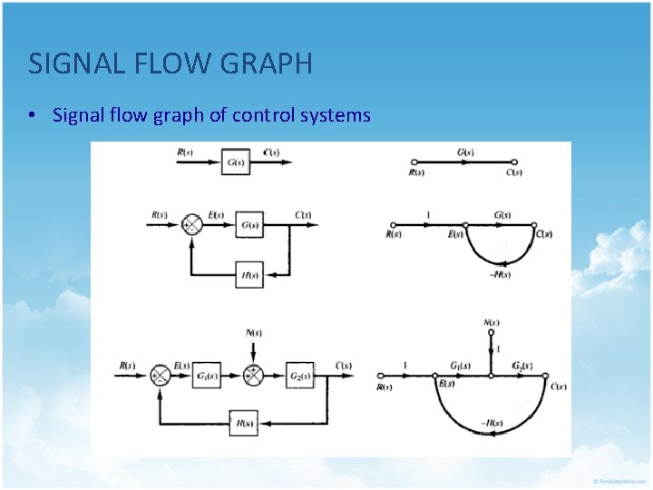
SIGNAL FLOW GRAPH • Signal flow graph of control systems

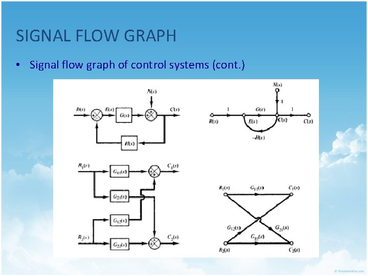
SIGNAL FLOW GRAPH • Signal flow graph of control systems (cont. )

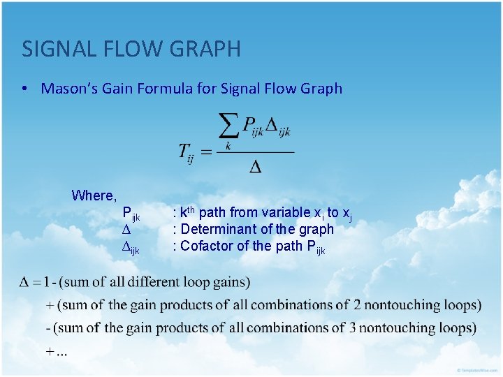
SIGNAL FLOW GRAPH • Mason’s Gain Formula for Signal Flow Graph Where, Pijk ∆ ∆ijk : kth path from variable xi to xj : Determinant of the graph : Cofactor of the path Pijk

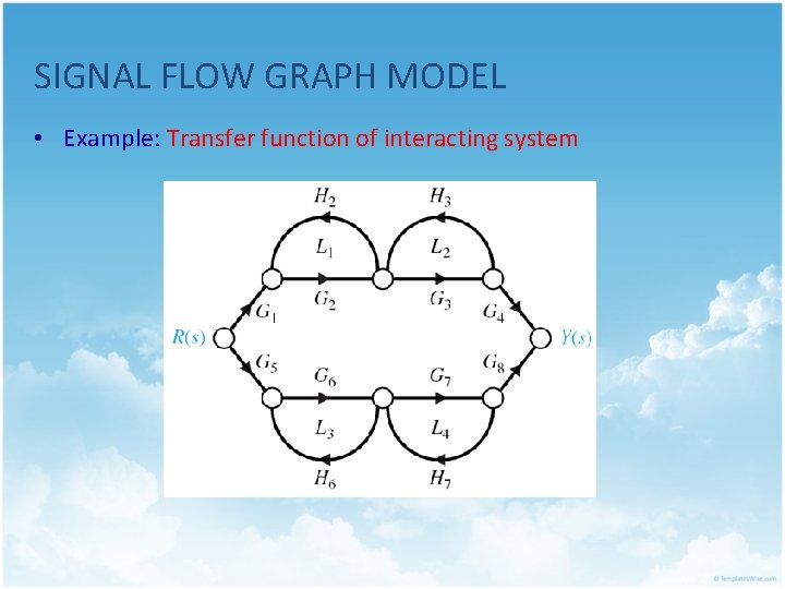
SIGNAL FLOW GRAPH MODEL • Example: Transfer function of interacting system

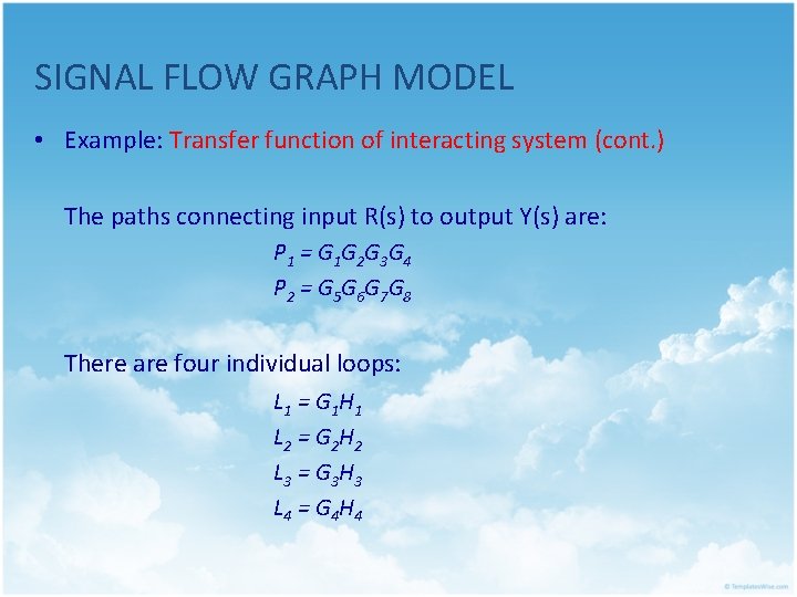
SIGNAL FLOW GRAPH MODEL • Example: Transfer function of interacting system (cont. ) The paths connecting input R(s) to output Y(s) are: P 1 = G 1 G 2 G 3 G 4 P 2 = G 5 G 6 G 7 G 8 There are four individual loops: L 1 = G 1 H 1 L 2 = G 2 H 2 L 3 = G 3 H 3 L 4 = G 4 H 4

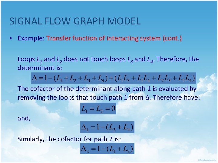
SIGNAL FLOW GRAPH MODEL • Example: Transfer function of interacting system (cont. ) Loops L 1 and L 2 does not touch loops L 3 and L 4. Therefore, the determinant is: The cofactor of the determinant along path 1 is evaluated by removing the loops that touch path 1 from ∆. Therefore have: and, Similarly, the cofactor for path 2 is:

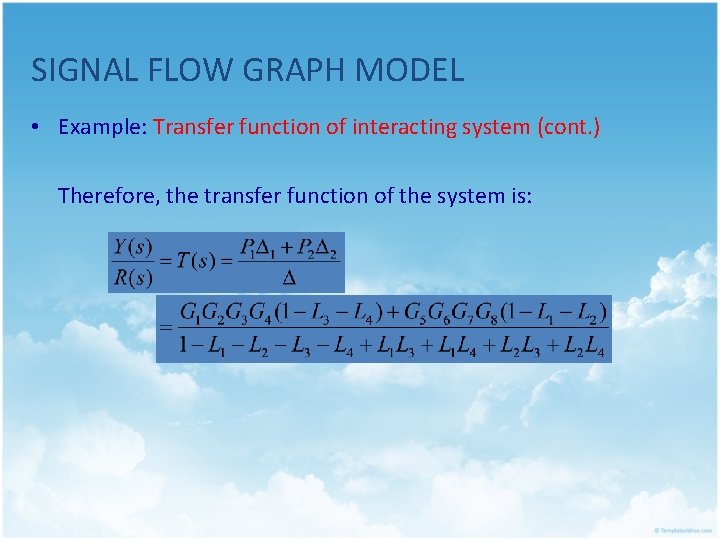
SIGNAL FLOW GRAPH MODEL • Example: Transfer function of interacting system (cont. ) Therefore, the transfer function of the system is:

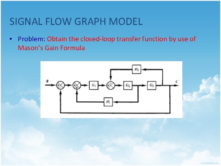
SIGNAL FLOW GRAPH MODEL • Problem: Obtain the closed-loop transfer function by use of Mason’s Gain Formula

FURTHER READING… • Chapter 3 i. ii. Dorf R. C. , Bishop R. H. (2001). Modern Control Systems (9 th Ed), Prentice Hall. Nise N. S. (2004). Control System Engineering (4 th Ed), John Wiley & Sons. • Chapter 5 i. Nise N. S. (2004). Control System Engineering (4 th Ed), John Wiley & Sons.

THE END…