Sparse Direct Methods on High Performance Computers X

Sparse Direct Methods on High Performance Computers X. Sherry Li xsli@lbl. gov http: //crd. lbl. gov/~xiaoye CS 267/ENg. C 233: Applications of Parallel Computing April 6, 2009

Sparse linear solvers v. Solving a system of linear equations Ax = b v. Iterative methods Ø A is not changed (read-only) Ø Key kernel: sparse matrix-vector multiply § Easier to optimize and parallelize Ø Low algorithmic complexity, but may not converge for hard problems v. Direct methods Ø A is modified (factorized) § Harder to optimize and parallelize Ø Numerically robust, but higher algorithmic complexity v. Often use direct method to precondition iterative method CS 267 2

Available sparse codes v. Survey of different types of factorization codes http: //crd. lbl. gov/~xiaoye/Super. LU/Sparse. Direct. Survey. pdf Ø LLT (s. p. d. ) Ø LDLT (symmetric indefinite) Ø LU (nonsymmetric) Ø QR (least squares) Ø Sequential, shared-memory (multicore), distributed-memory, outof-core v. Distributed-memory codes: usually MPI-based Ø Super. LU_DIST [Li/Demmel/Grigori] § accessible from PETSc, Trilinos Ø MUMPS, Pas. Ti. X, WSMP, . . . CS 267 3

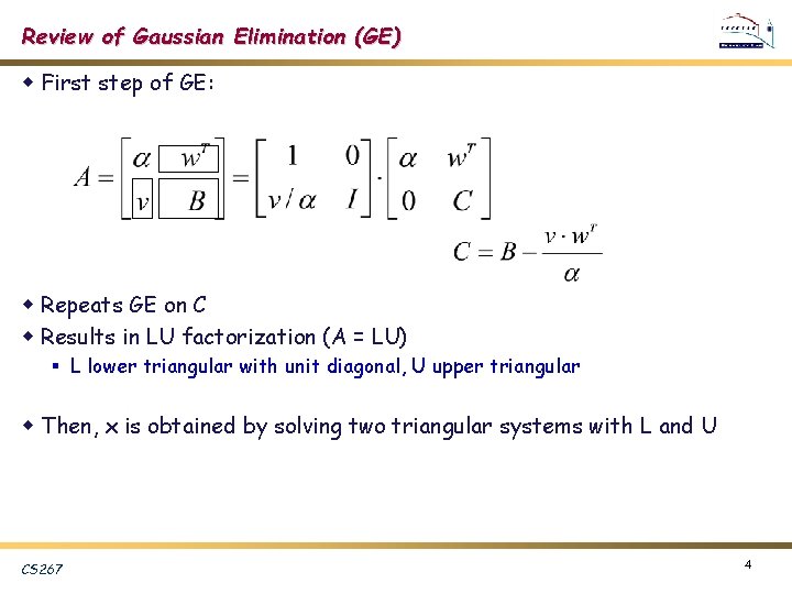
Review of Gaussian Elimination (GE) w First step of GE: w Repeats GE on C w Results in LU factorization (A = LU) § L lower triangular with unit diagonal, U upper triangular w Then, x is obtained by solving two triangular systems with L and U CS 267 4

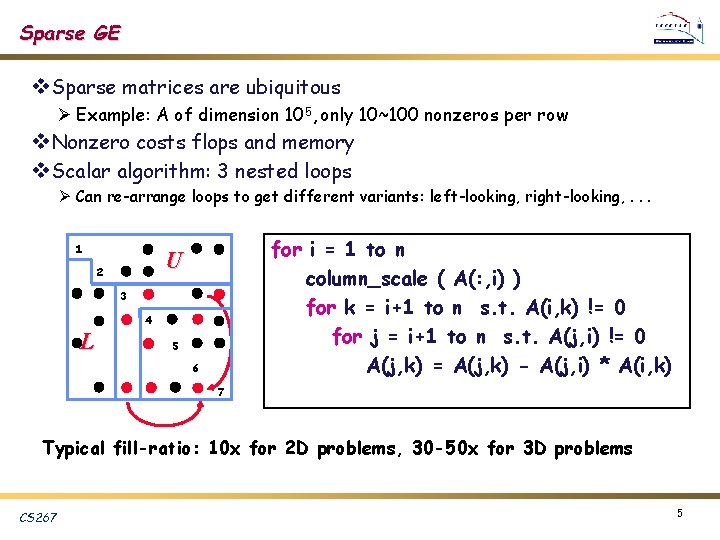
Sparse GE v. Sparse matrices are ubiquitous Ø Example: A of dimension 105, only 10~100 nonzeros per row v. Nonzero costs flops and memory v. Scalar algorithm: 3 nested loops Ø Can re-arrange loops to get different variants: left-looking, right-looking, . . . 1 for i = 1 to n column_scale ( A(: , i) ) for k = i+1 to n s. t. A(i, k) != 0 for j = i+1 to n s. t. A(j, i) != 0 A(j, k) = A(j, k) - A(j, i) * A(i, k) U 2 3 4 L 5 6 7 Typical fill-ratio: 10 x for 2 D problems, 30 -50 x for 3 D problems CS 267 5

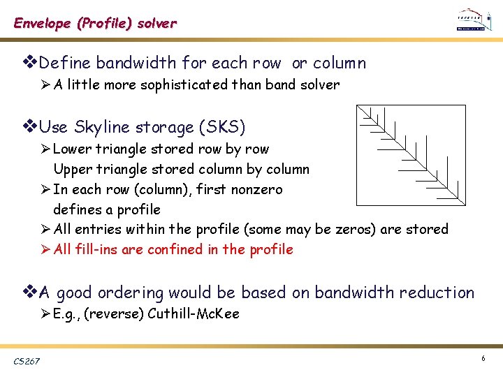
Envelope (Profile) solver v. Define bandwidth for each row or column Ø A little more sophisticated than band solver v. Use Skyline storage (SKS) Ø Lower triangle stored row by row Upper triangle stored column by column Ø In each row (column), first nonzero defines a profile Ø All entries within the profile (some may be zeros) are stored Ø All fill-ins are confined in the profile v. A good ordering would be based on bandwidth reduction Ø E. g. , (reverse) Cuthill-Mc. Kee CS 267 6

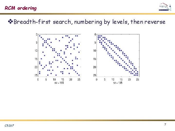
RCM ordering v. Breadth-first search, numbering by levels, then reverse CS 267 7

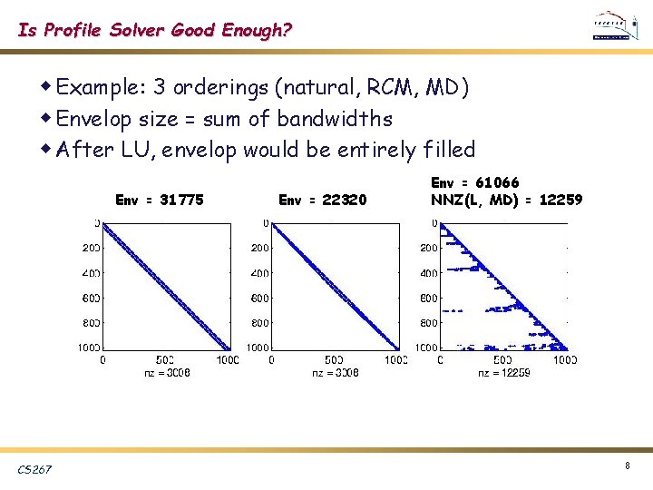
Is Profile Solver Good Enough? w Example: 3 orderings (natural, RCM, MD) w Envelop size = sum of bandwidths w After LU, envelop would be entirely filled Env = 31775 CS 267 Env = 22320 Env = 61066 NNZ(L, MD) = 12259 8

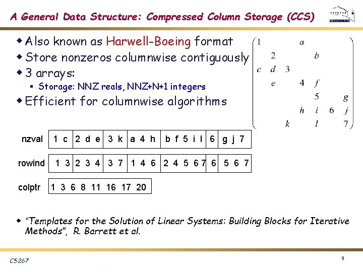
A General Data Structure: Compressed Column Storage (CCS) w Also known as Harwell-Boeing format w Store nonzeros columnwise contiguously w 3 arrays: § Storage: NNZ reals, NNZ+N+1 integers w Efficient for columnwise algorithms nzval rowind colptr 1 c 2 d e 3 k a 4 h b f 5 i l 6 g j 7 1 3 2 3 4 3 7 1 4 6 2 4 5 67 6 5 6 7 1 3 6 8 11 16 17 20 w “Templates for the Solution of Linear Systems: Building Blocks for Iterative Methods”, R. Barrett et al. CS 267 9

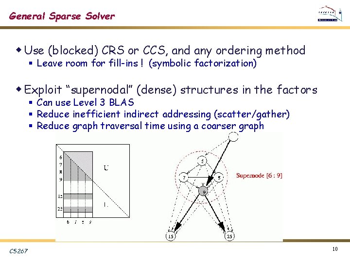
General Sparse Solver w Use (blocked) CRS or CCS, and any ordering method § Leave room for fill-ins ! (symbolic factorization) w Exploit “supernodal” (dense) structures in the factors § Can use Level 3 BLAS § Reduce inefficient indirect addressing (scatter/gather) § Reduce graph traversal time using a coarser graph CS 267 10

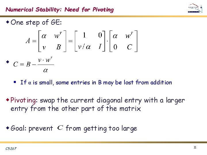
Numerical Stability: Need for Pivoting w One step of GE: w § If α is small, some entries in B may be lost from addition w Pivoting: swap the current diagonal entry with a larger entry from the other part of the matrix w Goal: prevent CS 267 from getting too large 11

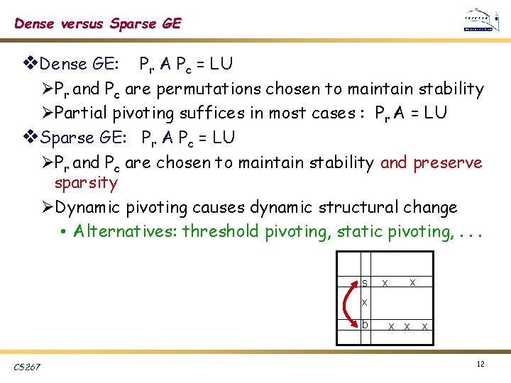
Dense versus Sparse GE v. Dense GE: Pr A Pc = LU ØPr and Pc are permutations chosen to maintain stability ØPartial pivoting suffices in most cases : Pr A = LU v. Sparse GE: Pr A Pc = LU ØPr and Pc are chosen to maintain stability and preserve sparsity ØDynamic pivoting causes dynamic structural change • Alternatives: threshold pivoting, static pivoting, . . . s x x x b CS 267 x x x 12

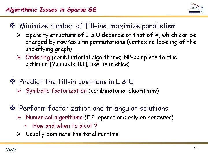
Algorithmic Issues in Sparse GE v Minimize number of fill-ins, maximize parallelism Ø Sparsity structure of L & U depends on that of A, which can be changed by row/column permutations (vertex re-labeling of the underlying graph) Ø Ordering (combinatorial algorithms; NP-complete to find optimum [Yannakis ’ 83]; use heuristics) v Predict the fill-in positions in L & U Ø Symbolic factorization (combinatorial algorithms) v Perform factorization and triangular solutions Ø Numerical algorithms (F. P. operations only on nonzeros) • How and when to pivot ? Ø Usually dominate the total runtime CS 267 13

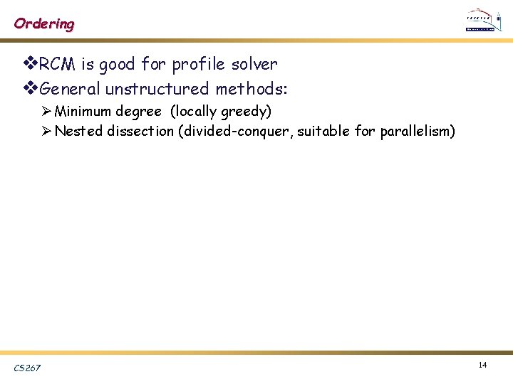
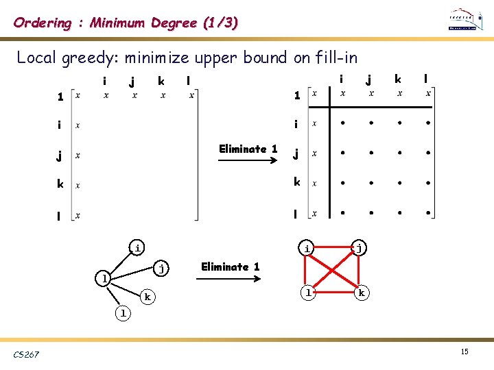
Ordering v. RCM is good for profile solver v. General unstructured methods: Ø Minimum degree (locally greedy) Ø Nested dissection (divided-conquer, suitable for parallelism) CS 267 14

Ordering : Minimum Degree (1/3) Local greedy: minimize upper bound on fill-in i j k i l 1 1 i i Eliminate 1 j k l l j 1 k k l j k i j l k Eliminate 1 l CS 267 15

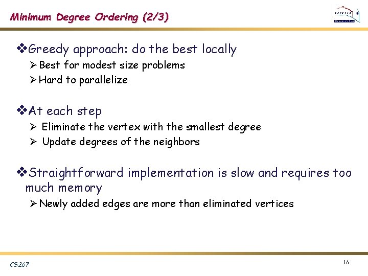
Minimum Degree Ordering (2/3) v. Greedy approach: do the best locally Ø Best for modest size problems Ø Hard to parallelize v. At each step Ø Eliminate the vertex with the smallest degree Ø Update degrees of the neighbors v. Straightforward implementation is slow and requires too much memory Ø Newly added edges are more than eliminated vertices CS 267 16

Minimum Degree Ordering (3/3) v. Use quotient graph as a compact representation [George/Liu ’ 78] v. Collection of cliques resulting from the eliminated vertices affects the degree of an uneliminated vertex v. Represent each connected component in the eliminated subgraph by a single “supervertex” v. Storage required to implement QG model is bounded by size of A v. Large body of literature on implementation variants Ø Tinney/Walker `67, George/Liu `79, Liu `85, Amestoy/Davis/Duff `94, Ashcraft `95, Duff/Reid `95, et al. , . . CS 267 17

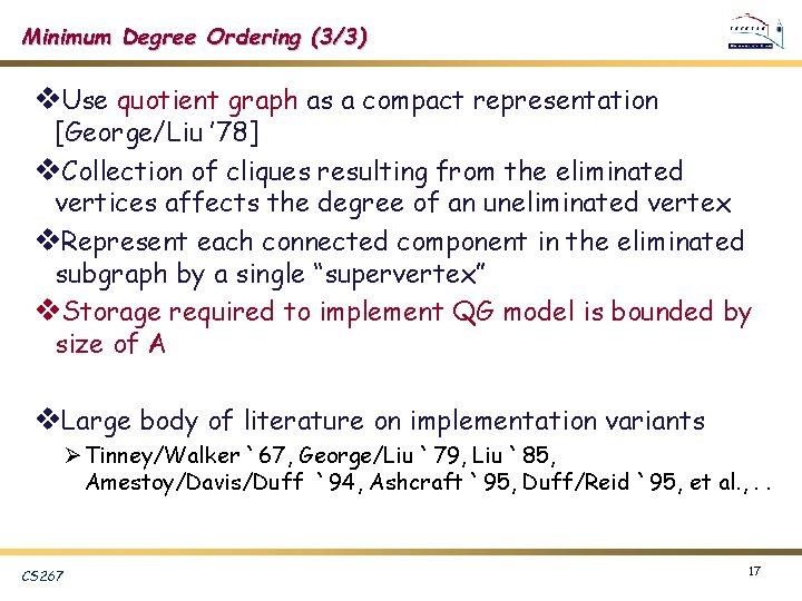
Nested Dissection Ordering (1/3) v. Model problem: discretized system Ax = b from certain PDEs, e. g. , 5 -point stencil on n x n grid, N = n^2 v. Theorem: ND ordering gave optimal complexity in exact arithmetic [George ’ 73, Hoffman/Martin/Rose] Ø 2 D (kxk = N grids): O(N log. N) memory, O(N 3/2) operations Ø 3 D (kxkxk = N grids): O(N 4/3) memory, O(N 2) operations CS 267 18

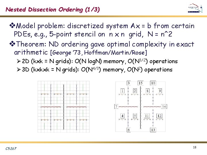
ND Ordering (2/3) w Generalized nested dissection [Lipton/Rose/Tarjan ’ 79] § Global graph partitioning: top-down, divide-and-conqure § Best for largest problems § Parallel codes available: e. g. , Par. Metis, Scotch § First level A S B § Recurse on A and B w Goal: find the smallest possible separator S at each level § Multilevel schemes: Chaco [Hendrickson/Leland `94], Metis [Karypis/Kumar `95] § Spectral bisection [Simon et al. `90 -`95] § Geometric and spectral bisection [Chan/Gilbert/Teng `94] CS 267 19

ND Ordering (3/3) CS 267 20

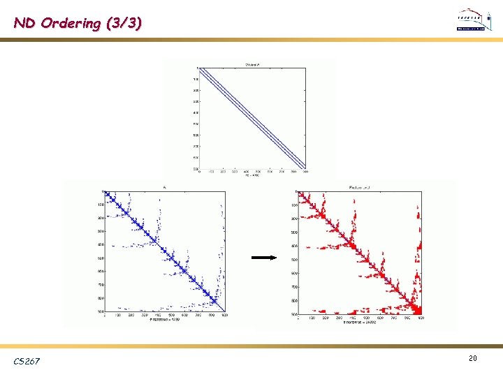
Ordering for LU (unsymmetric) v Can use a symmetric ordering on a symmetrized matrix Ø Case of partial pivoting (sequential Super. LU): Use ordering based on ATA Ø Case of static pivoting (Super. LU_DIST): Use ordering based on AT+A v Can find better ordering based solely on A Ø Diagonal Markowitz [Amestoy/Li/Ng ‘ 06] § Similar to minimum degree, but without symmetrization Ø Hypergraph partition [Boman, Grigori, et al. , ‘ 09] § Similar to ND on ATA, but no need to compute ATA CS 267 21

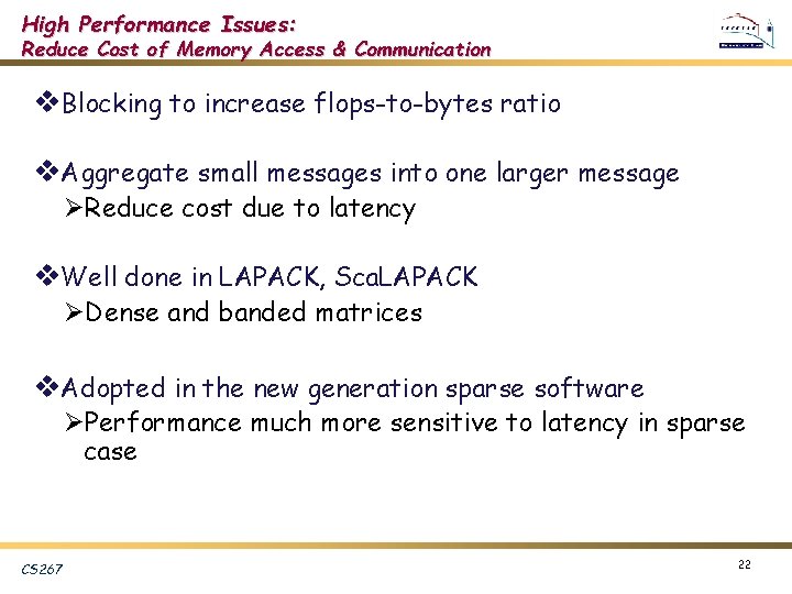
High Performance Issues: Reduce Cost of Memory Access & Communication v. Blocking to increase flops-to-bytes ratio v. Aggregate small messages into one larger message ØReduce cost due to latency v. Well done in LAPACK, Sca. LAPACK ØDense and banded matrices v. Adopted in the new generation sparse software ØPerformance much more sensitive to latency in sparse case CS 267 22

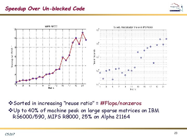
Speedup Over Un-blocked Code v. Sorted in increasing “reuse ratio” = #Flops/nonzeros v. Up to 40% of machine peak on large sparse matrices on IBM RS 6000/590, MIPS R 8000, 25% on Alpha 21164 CS 267 23

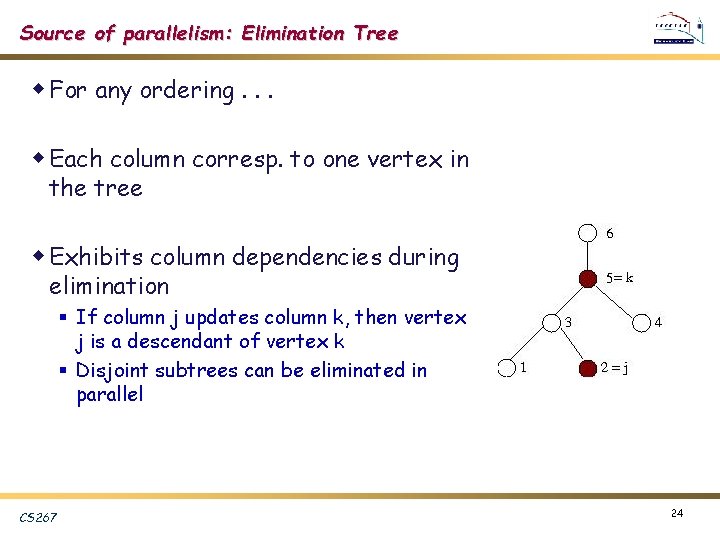
Source of parallelism: Elimination Tree w For any ordering. . . w Each column corresp. to one vertex in the tree w Exhibits column dependencies during elimination § If column j updates column k, then vertex j is a descendant of vertex k § Disjoint subtrees can be eliminated in parallel CS 267 24

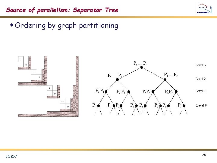
Source of parallelism: Separator Tree w Ordering by graph partitioning CS 267 25

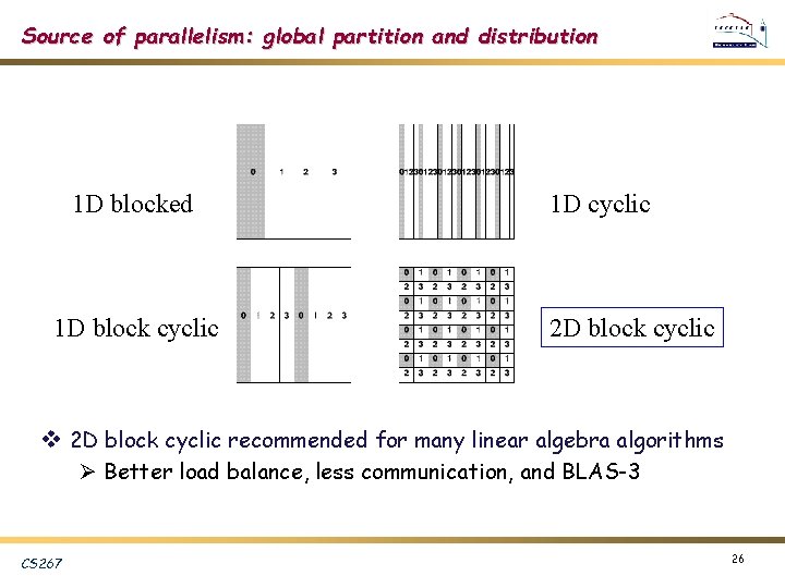
Source of parallelism: global partition and distribution 1 D blocked 1 D block cyclic 1 D cyclic 2 D block cyclic v 2 D block cyclic recommended for many linear algebra algorithms Ø Better load balance, less communication, and BLAS-3 CS 267 26

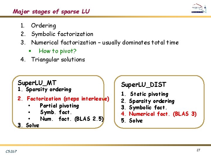
Major stages of sparse LU 1. Ordering 2. Symbolic factorization 3. Numerical factorization – usually dominates total time § How to pivot? 4. Triangular solutions Super. LU_MT 1. Sparsity ordering 2. Factorization (steps interleave) Partial pivoting • Symb. fact. • Num. fact. (BLAS 2. 5) • 3. Solve CS 267 Super. LU_DIST 1. 2. 3. 4. 5. Static pivoting Sparsity ordering Symbolic fact. Numerical fact. (BLAS 3) Solve 27

[Li/Demmel/Gilbert] Super. LU_MT v. Pthreads or Open. MP v. Left looking -- many more reads than writes v. Use shared task queue to schedule ready columns in the elimination tree (bottom up) P 1 P 2 U A L DONE CS 267 BUSY NOT TOUCHED 28

Super. LU_DIST [Li/Demmel/Grigori] v. MPI v. Right looking -- many more writes than reads v. Global 2 D block cyclic layout v. One step look-ahead to overlap comm. & comp. Matrix Process mesh 0 1 2 0 3 4 5 3 0 1 2 0 3 4 5 3 0 1 2 0 1 0 1 2 3 4 5 ACTIVE CS 267 29

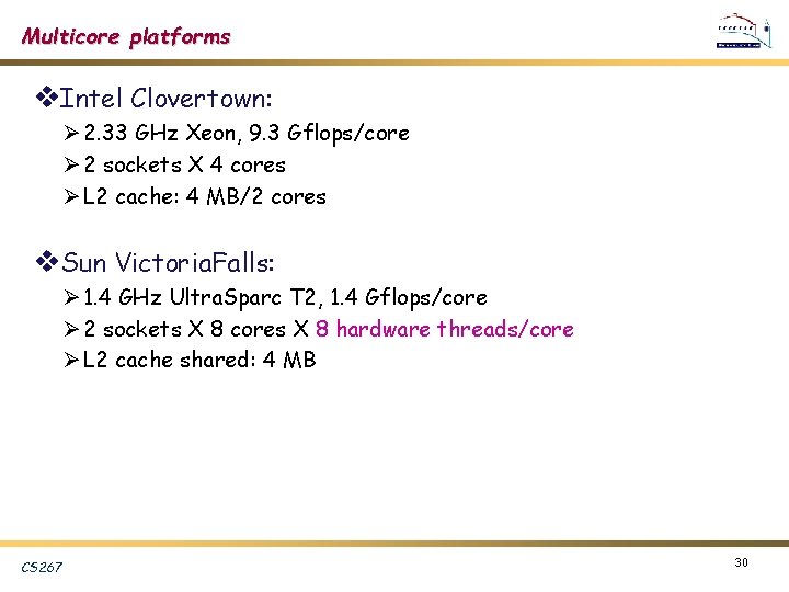
Multicore platforms v. Intel Clovertown: Ø 2. 33 GHz Xeon, 9. 3 Gflops/core Ø 2 sockets X 4 cores Ø L 2 cache: 4 MB/2 cores v. Sun Victoria. Falls: Ø 1. 4 GHz Ultra. Sparc T 2, 1. 4 Gflops/core Ø 2 sockets X 8 cores X 8 hardware threads/core Ø L 2 cache shared: 4 MB CS 267 30

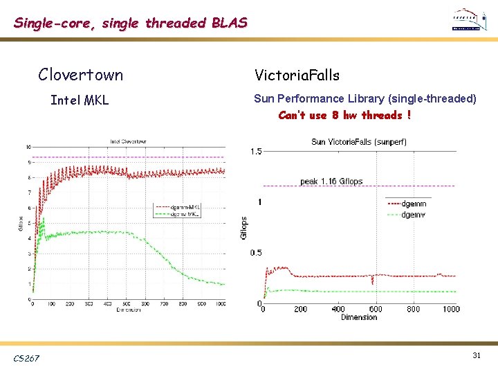
Single-core, single threaded BLAS Clovertown Intel MKL CS 267 Victoria. Falls Sun Performance Library (single-threaded) Can’t use 8 hw threads ! 31

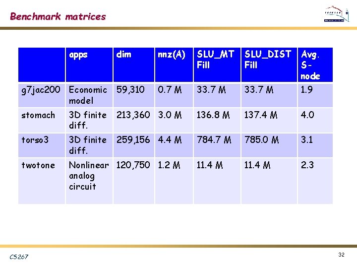
Benchmark matrices apps dim nnz(A) SLU_MT Fill SLU_DIST Fill Avg. Snode g 7 jac 200 Economic model 59, 310 0. 7 M 33. 7 M 1. 9 stomach 3 D finite diff. 213, 360 3. 0 M 136. 8 M 137. 4 M 4. 0 torso 3 3 D finite diff. 259, 156 4. 4 M 784. 7 M 785. 0 M 3. 1 twotone Nonlinear 120, 750 1. 2 M analog circuit 11. 4 M 2. 3 CS 267 32

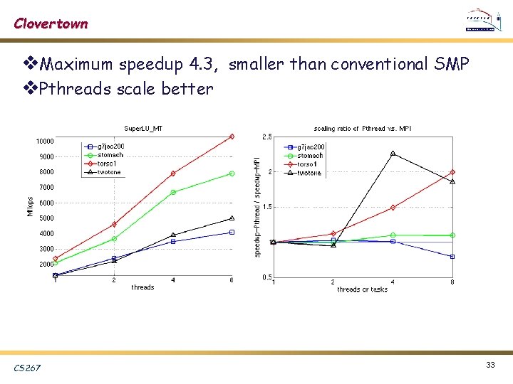
Clovertown v. Maximum speedup 4. 3, smaller than conventional SMP v. Pthreads scale better CS 267 33

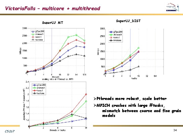
Victoria. Falls – multicore + multithread Super. LU_MT Super. LU_DIST ØPthreads more robust, scale better ØMPICH crashes with large #tasks, mismatch between coarse and fine grain models CS 267 34

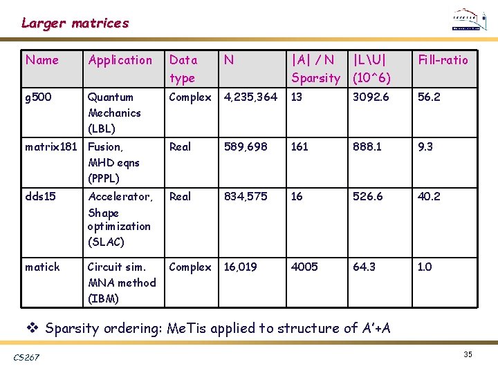
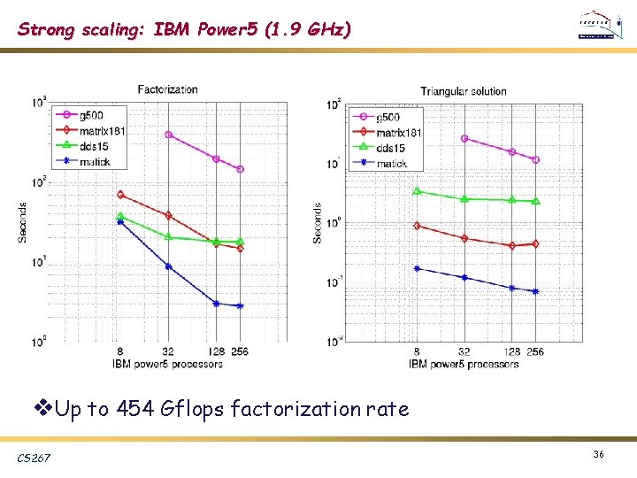
Larger matrices Name Application Data type N |A| / N |LU| Sparsity (10^6) Fill-ratio g 500 Quantum Mechanics (LBL) Complex 4, 235, 364 13 3092. 6 56. 2 matrix 181 Fusion, MHD eqns (PPPL) Real 589, 698 161 888. 1 9. 3 dds 15 Accelerator, Shape optimization (SLAC) Real 834, 575 16 526. 6 40. 2 matick Circuit sim. MNA method (IBM) Complex 16, 019 4005 64. 3 1. 0 v Sparsity ordering: Me. Tis applied to structure of A’+A CS 267 35

Strong scaling: IBM Power 5 (1. 9 GHz) v. Up to 454 Gflops factorization rate CS 267 36

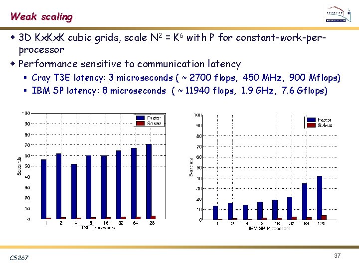
Weak scaling w 3 D Kx. K cubic grids, scale N 2 = K 6 with P for constant-work-perprocessor w Performance sensitive to communication latency § Cray T 3 E latency: 3 microseconds ( ~ 2700 flops, 450 MHz, 900 Mflops) § IBM SP latency: 8 microseconds ( ~ 11940 flops, 1. 9 GHz, 7. 6 Gflops) CS 267 37

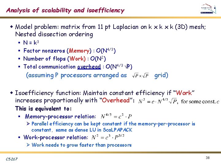
Analysis of scalability and isoefficiency w Model problem: matrix from 11 pt Laplacian on k x k (3 D) mesh; Nested dissection ordering § § N = k 3 Factor nonzeros (Memory) : O(N 4/3) Number of flops (Work) : O(N 2) Total communication overhead : O(N 4/3 P) (assuming P processors arranged as grid) w Isoefficiency function: Maintain constant efficiency if “Work” increases proportionally with “Overhead”: This is equivalent to: § Memory-processor relation: Ø Parallel efficiency can be kept constant if the memory-per-processor is constant, same as dense LU in Sca. LPAPACK § Work-processor relation: Ø Work needs to grow faster than processors CS 267 38

Summary v. Important kernel for science and engineering applications, used in practice on a regular basis v. Good implementation on high-performance machines requires a large set of tools from CS and NLA v. Performance more sensitive to latency than dense case CS 267 39

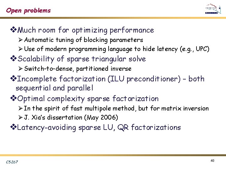
Open problems v. Much room for optimizing performance Ø Automatic tuning of blocking parameters Ø Use of modern programming language to hide latency (e. g. , UPC) v. Scalability of sparse triangular solve Ø Switch-to-dense, partitioned inverse v. Incomplete factorization (ILU preconditioner) – both sequential and parallel v. Optimal complexity sparse factorization Ø In the spirit of fast multipole method, but for matrix inversion Ø J. Xia’s dissertation (May 2006) v. Latency-avoiding sparse LU, QR factorizations CS 267 40

Extra Slides CS 267 41

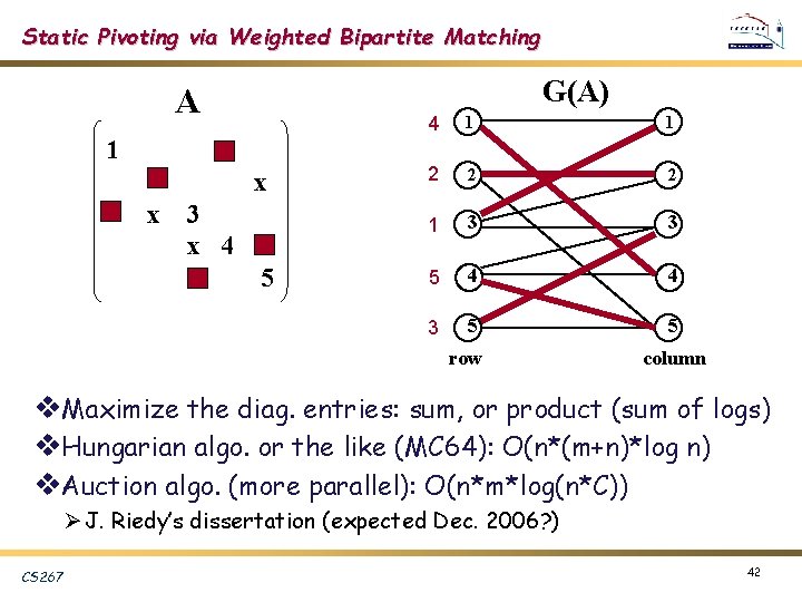
Static Pivoting via Weighted Bipartite Matching G(A) A 1 x x 3 x 4 5 4 1 1 2 2 2 1 3 3 5 4 4 3 5 5 row column v. Maximize the diag. entries: sum, or product (sum of logs) v. Hungarian algo. or the like (MC 64): O(n*(m+n)*log n) v. Auction algo. (more parallel): O(n*m*log(n*C)) Ø J. Riedy’s dissertation (expected Dec. 2006? ) CS 267 42

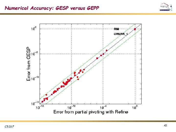
Numerical Accuracy: GESP versus GEPP CS 267 43

Parallel Symbolic Factorization [Grigori/Demmel/Li ‘ 06] v. Parallel ordering with Par. METIS on G(A’+A) v. Separator tree (binary) to guide computation ØEach step: one row of U, one column of L ØWithin each separator: 1 D block cyclic distribution ØSend necessary contribution to parent processor v. Results: ØReasonable speedup: up to 6 x Ø 5 x reduction in maximum per-processor memory needs ØNeed improve memory balance CS 267 44

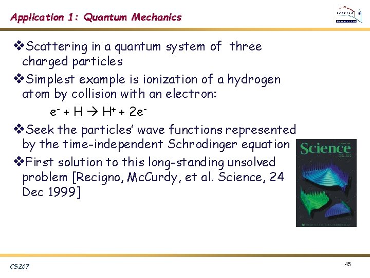
Application 1: Quantum Mechanics v. Scattering in a quantum system of three charged particles v. Simplest example is ionization of a hydrogen atom by collision with an electron: e- + H H+ + 2 ev. Seek the particles’ wave functions represented by the time-independent Schrodinger equation v. First solution to this long-standing unsolved problem [Recigno, Mc. Curdy, et al. Science, 24 Dec 1999] CS 267 45

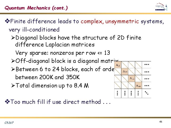
Quantum Mechanics (cont. ) v. Finite difference leads to complex, unsymmetric systems, very ill-conditioned ØDiagonal blocks have the structure of 2 D finite difference Laplacian matrices Very sparse: nonzeros per row <= 13 ØOff-diagonal block is a diagonal matrix ØBetween 6 to 24 blocks, each of order between 200 K and 350 K ØTotal dimension up to 8. 4 M v. Too much fill if use direct method. . . CS 267 46

Super. LU_DIST as Preconditioner v. Super. LU_DIST as block-diagonal preconditioner for CGS iteration M-1 A x = M-1 b M = diag(A 11, A 22, A 33, …) v. Run multiple Super. LU_DIST simultaneously for diagonal blocks v. No pivoting, nor iterative refinement v 12 to 35 CGS iterations @ 1 ~ 2 minute/iteration using 64 IBM SP processors Total time: 0. 5 to a few hours CS 267 47

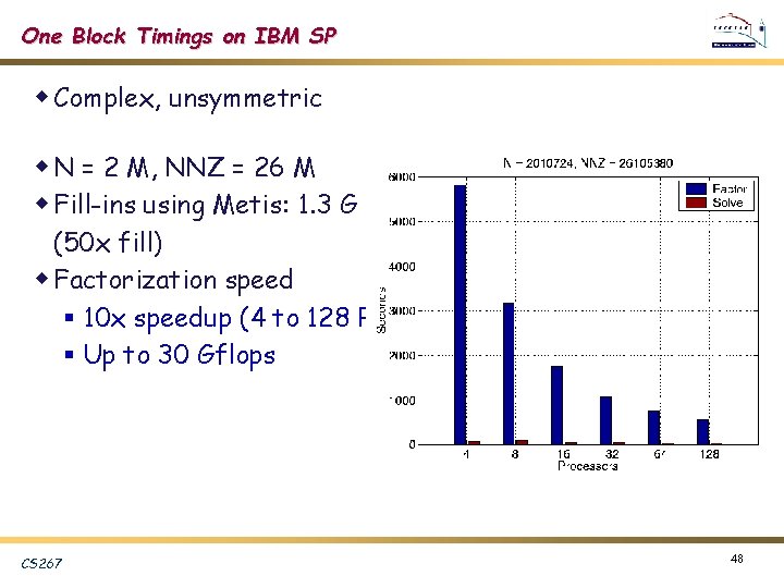
One Block Timings on IBM SP w Complex, unsymmetric w N = 2 M, NNZ = 26 M w Fill-ins using Metis: 1. 3 G (50 x fill) w Factorization speed § 10 x speedup (4 to 128 P) § Up to 30 Gflops CS 267 48

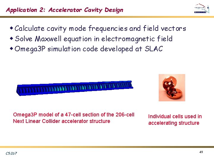
Application 2: Accelerator Cavity Design w Calculate cavity mode frequencies and field vectors w Solve Maxwell equation in electromagnetic field w Omega 3 P simulation code developed at SLAC Omega 3 P model of a 47 -cell section of the 206 -cell Next Linear Collider accelerator structure CS 267 Individual cells used in accelerating structure 49

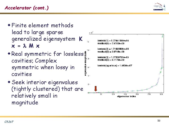
Accelerator (cont. ) w Finite element methods lead to large sparse generalized eigensystem K x = M x w Real symmetric for lossless cavities; Complex symmetric when lossy in cavities w Seek interior eigenvalues (tightly clustered) that are relatively small in magnitude CS 267 50

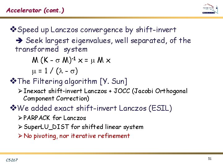
Accelerator (cont. ) v. Speed up Lanczos convergence by shift-invert Seek largest eigenvalues, well separated, of the transformed system M (K - M)-1 x = M x = 1 / ( - ) v. The Filtering algorithm [Y. Sun] Ø Inexact shift-invert Lanczos + JOCC (Jacobi Orthogonal Component Correction) v. We added exact shift-invert Lanczos (ESIL) Ø PARPACK for Lanczos Ø Super. LU_DIST for shifted linear system Ø No pivoting, nor iterative refinement CS 267 51

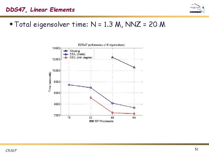
DDS 47, Linear Elements w Total eigensolver time: N = 1. 3 M, NNZ = 20 M CS 267 52

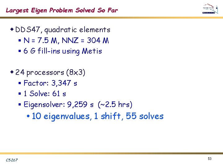
Largest Eigen Problem Solved So Far w DDS 47, quadratic elements § N = 7. 5 M, NNZ = 304 M § 6 G fill-ins using Metis w 24 processors (8 x 3) § Factor: 3, 347 s § 1 Solve: 61 s § Eigensolver: 9, 259 s (~2. 5 hrs) 10 eigenvalues, 1 shift, 55 solves CS 267 53

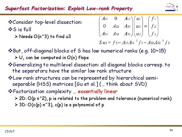
Superfast Factorization: Exploit Low-rank Property v. Consider top-level dissection: v. S is full Ø Needs O(n^3) to find u 3 v. But, off-diagonal blocks of S has low numerical ranks (e. g. 10~15) Ø U 3 can be computed in O(n) flops v. Generalizing to multilevel dissection: all diagonal blocks corresp. to the separators have the similar low rank structure v. Low rank structures can be represented by hierarchical semiseparable (HSS) matrices [Gu et al. ] (… think about SVD) v. Factorization complexity … essentially linear Ø 2 D: O(p n^2), p is related to the problem and tolerance (numerical rank) Ø 3 D: O(c(p) n^3), c(p) is a polynomial of p CS 267 54

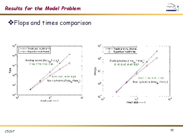
Results for the Model Problem v. Flops and times comparison CS 267 55

Research Issues v. Analysis of 3 D problems, and complex geometry v. Larger tolerance preconditioner (another type of ILU) Ø If SPD, want all the low rank structures to remain SPD (“Schur-monotonic” talk by M. Gu, Wed, 5/3) v. Performance tuning for many small dense matrices (e. g. 10~20) v. Switching level in a hybrid solver Ø Benefits show up only for large enough mesh v. Local ordering of unknowns Ø E. g. : node ordering within a separator affects numerical ranks v. Parallel algorithm and implementation CS 267 56