Simulating neural networks with Romain Brette romain bretteens
")
Simulating neural networks with Romain Brette (romain. brette@ens. fr)

SPIKING NEURON MODELS

Spiking neuron models Input = N spike trains Output = 1 spike train A neuron model is defined by: • what happens when a spike is received • the condition for spiking • what happens when a spike is produced • what happens between spikes discrete events continuous dynamics

The membrane equation outside =1/R Vm inside Iinj membrane time constant (typically 3 -100 ms)
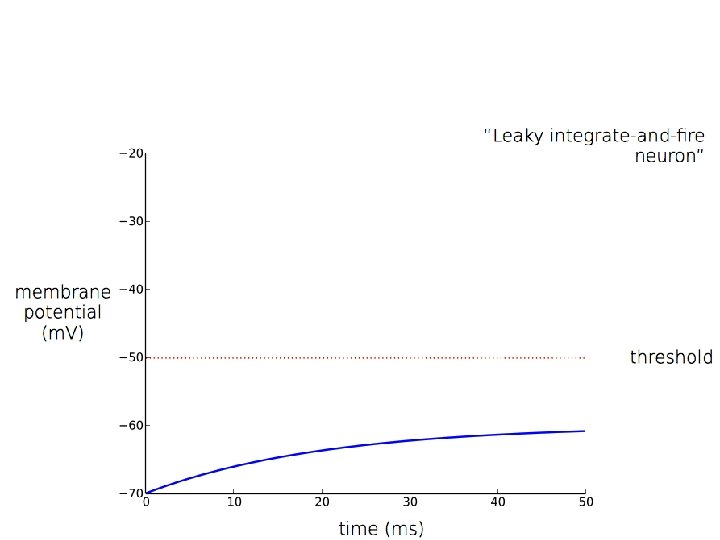
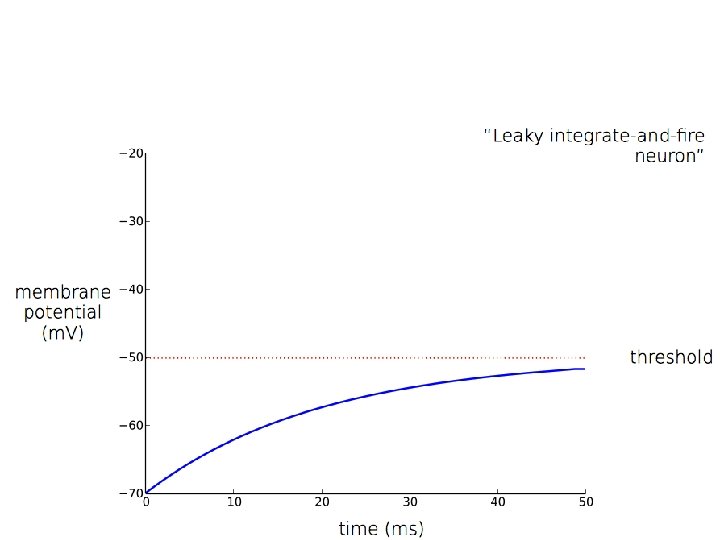
 then: neuron spikes and V→Vr (reset)")
Spiking: If V = Vt (threshold) then: neuron spikes and V→Vr (reset)

The Hodgkin-Huxley model Model of the space clamped giant squid axon Hodgkin & Huxley (Nobel prize 1963)
 spike threshold temporal")
Synaptic integration action potential or « spike » postsynaptic potential (PSP) spike threshold temporal integration
")
Synaptic currents synapse synaptic current postsynaptic neuron Is(t)

Idealized synapse • Total charge • Opens for a short duration • Vm increases by Q/C at t=0 EL
 open presynaptic")
A more realistic synapse model ionic channel conductance synaptic reversal potential gs(t) open presynaptic spike closed
![Example of kinetic model • Stochastic transitions between open and closed α[L] C ⇄β](http://slidetodoc.com/presentation_image_h2/c3d4cc1d024f0f4f2b0f2e93962c969e/image-13.jpg "Example of kinetic model • Stochastic transitions between open and closed α[L] C ⇄β")
Example of kinetic model • Stochastic transitions between open and closed α[L] C ⇄β O opening rate, proportional to concentration constant closing rate Macroscopic equation (many channels): proportion of open channels gs(t)=x(t)*gmax Assuming neurotransmitter are present for a very short duration: τs=1/β
 threshold reset")
General spiking neuron models evolution of state variables presynaptic spike (synapse i) threshold reset tran smi Typically: V=Vt: V→Vr ssio n dela y

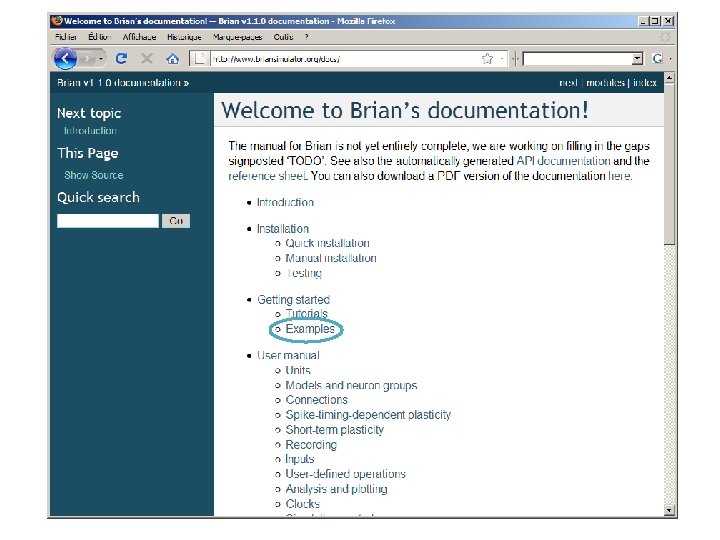
http: //www. briansimulator. org

The spirit of “A simulator should not only save the time of processors, but also the time of scientists” scientist computer Writing code often takes more time than running it Goals: • Quick model coding • Flexible models are defined by equations (rather than pre-defined) Goodman, D. and R. Brette (2009). The Brian simulator. Front Neurosci doi: 10. 3389/neuro. 01. 026. 2009.

Who is Brian? briansimulator. org


Example: current-frequency curve from brian import * N = 1000 tau = 10 * ms eqs = ''' dv/dt=(v 0 -v)/tau : volt v 0 : volt ''' group = Neuron. Group(N, model=eqs, threshold=10 * m. V, reset=0 * m. V, refractory=5 * ms) group. v = 0 * m. V group. v 0 = linspace(0 * m. V, 20 * m. V, N) counter = Spike. Counter(group) duration = 5 * second run(duration) plot(group. v 0 / m. V, counter. count / duration) show()

Example: a fully connected network from brian import * tau = 10 * ms v 0 = 11 * m. V N = 20 w =. 1 * m. V group = Neuron. Group(N, model='dv/dt=(v 0 -v)/tau : volt', threshold=10 * m. V, reset=0 * m. V) W = Connection(group, 'v', weight=w) group. v = rand(N) * 10 * m. V S = Spike. Monitor(group) run(300 * ms) raster_plot(S) show()

Example: a fully connected network from brian import * tau = 10 * ms v 0 = 11 * m. V N = 20 w =. 1 * m. V group = Neuron. Group(N, model='dv/dt=(v 0 -v)/tau : volt', threshold=10 * m. V, reset=0 * m. V) W = Connection(group, 'v', weight=w) group. v = rand(N) * 10 * m. V S = Spike. Monitor(group) run(300 * ms) raster_plot(S) show() R. E. Mirollo and S. H. Strogatz. Synchronization of pulse-coupled biological oscillators. SIAM Journal on Applied Mathematics 50, 1645 -1662 (1990).

Example 2: a ring of IF neurons from brian import * tau = 10 * ms v 0 = 11 * m. V N = 20 w = 1 * m. V ring = Neuron. Group(N, model='dv/dt=(v 0 -v)/tau : volt', threshold=10 * m. V, reset=0 * m. V) W = Connection(ring, 'v') for i in range(N): W[i, (i + 1) % N] = w ring. v = rand(N) * 10 * m. V S = Spike. Monitor(ring) run(300 * ms) raster_plot(S) show()

Example 2: a ring of IF neurons from brian import * tau = 10 * ms v 0 = 11 * m. V N = 20 w = 1 * m. V ring = Neuron. Group(N, model='dv/dt=(v 0 -v)/tau : volt', threshold=10 * m. V, reset=0 * m. V) W = Connection(ring, 'v') for i in range(N): W[i, (i + 1) % N] = w ring. v = rand(N) * 10 * m. V S = Spike. Monitor(ring) run(300 * ms) raster_plot(S) show()

Example 3: a noisy ring from brian import * tau = 10 * ms sigma =. 5 N = 100 mu = 2 eqs = """ dv/dt=mu/tau+sigma/tau**. 5*xi : 1 """ group = Neuron. Group(N, model=eqs, threshold=1, reset=0) C = Connection(group, 'v') for i in range(N): C[i, (i + 1) % N] = -1 S = Spike. Monitor(group) trace = State. Monitor(group, 'v', record=True) run(500 * ms) subplot(211) raster_plot(S) subplot(212) plot(trace. times / ms, trace[0]) show()

Example 3: a noisy ring from brian import * tau = 10 * ms sigma =. 5 N = 100 mu = 2 eqs = """ dv/dt=mu/tau+sigma/tau**. 5*xi : 1 """ group = Neuron. Group(N, model=eqs, threshold=1, reset=0) C = Connection(group, 'v') for i in range(N): C[i, (i + 1) % N] = -1 S = Spike. Monitor(group) trace = State. Monitor(group, 'v', record=True) run(500 * ms) subplot(211) raster_plot(S) subplot(212) plot(trace. times / ms, trace[0]) show()

Example 4: topographic connections from brian import * tau = 10 * ms N = 100 v 0 = 5 * m. V sigma = 4 * m. V group = Neuron. Group(N, model='dv/dt=(v 0 -v)/tau + sigma*xi/tau**. 5 : volt', threshold=10 * m. V, reset=0 * m. V) C = Connection(group, 'v', weight=lambda i, j: . 4 * m. V * cos(2. * pi * (i - j) * 1. / N)) S = Spike. Monitor(group) R = Population. Rate. Monitor(group) group. v = rand(N) * 10 * m. V run(5000 * ms) subplot(211) raster_plot(S) subplot(223) imshow(C. W. todense(), interpolation='nearest') title('Synaptic connections') subplot(224) plot(R. times / ms, R. smooth_rate(2 * ms, filter='flat')) title('Firing rate') show()

Example 4: topographic connections from brian import * tau = 10 * ms N = 100 v 0 = 5 * m. V sigma = 4 * m. V group = Neuron. Group(N, model='dv/dt=(v 0 -v)/tau + sigma*xi/tau**. 5 : volt', threshold=10 * m. V, reset=0 * m. V) C = Connection(group, 'v', weight=lambda i, j: . 4 * m. V * cos(2. * pi * (i - j) * 1. / N)) S = Spike. Monitor(group) R = Population. Rate. Monitor(group) group. v = rand(N) * 10 * m. V run(5000 * ms) subplot(211) raster_plot(S) subplot(223) imshow(C. W. todense(), interpolation='nearest') title('Synaptic connections') subplot(224) plot(R. times / ms, R. smooth_rate(2 * ms, filter='flat')) title('Firing rate') show()

Example 5: random network from brian import * taum taue taui Ee = Ei = = 20 * msecond = 5 * msecond = 10 * msecond 60 * mvolt -80 * mvolt eqs = ''' dv/dt = (-v+ge*(Ee-v)+gi*(Ei-v))*(1. /taum) : volt dge/dt = -ge/taue : 1 dgi/dt = -gi/taui : 1''' P = Neuron. Group(4000, model=eqs, threshold=10 * mvolt , reset=0 * mvolt, refractory=5 * msecond) Pe = P. subgroup(3200) Pi = P. subgroup(800) we = 0. 6 wi = 6. 7 Ce = Connection(Pe, P, 'ge', weight=we, sparseness=0. 02) Ci = Connection(Pi, P, 'gi', weight=wi, sparseness=0. 02) P. v = (randn(len(P)) * 5 - 5) * mvolt P. ge = randn(len(P)) * 1. 5 + 4 P. gi = randn(len(P)) * 12 + 20 S = Spike. Monitor(P) run(1 * second) raster_plot(S) show()

Example 5: random network from brian import * taum taue taui Ee = Ei = = 20 * msecond = 5 * msecond = 10 * msecond 60 * mvolt -80 * mvolt eqs = ''' dv/dt = (-v+ge*(Ee-v)+gi*(Ei-v))*(1. /taum) : volt dge/dt = -ge/taue : 1 dgi/dt = -gi/taui : 1''' P = Neuron. Group(4000, model=eqs, threshold=10 * mvolt , reset=0 * mvolt, refractory=5 * msecond) Pe = P. subgroup(3200) Pi = P. subgroup(800) we = 0. 6 wi = 6. 7 Ce = Connection(Pe, P, 'ge', weight=we, sparseness=0. 02) Ci = Connection(Pi, P, 'gi', weight=wi, sparseness=0. 02) P. v = (randn(len(P)) * 5 - 5) * mvolt P. ge = randn(len(P)) * 1. 5 + 4 P. gi = randn(len(P)) * 12 + 20 S = Spike. Monitor(P) run(1 * second) raster_plot(S) show()
 Postsynaptic")
Synaptic plasticity c pre post: potentiation post pre: depression Dan & Poo (2006) Postsynaptic spike pti a yn s e Pr ike p s (STDP = Spike-Timing. Dependent Plasticity)

Phenomenological model Presynaptic spike: Postsynaptic spike:
 eqs_stdp=''' d. A_pre/dt=-A_pre/tau_pre : 1 d. A_post/dt=-A_post/tau_post")
Synaptic plasticity with Brian synapses=Connection(input, neurons, 'ge') eqs_stdp=''' d. A_pre/dt=-A_pre/tau_pre : 1 d. A_post/dt=-A_post/tau_post : 1 ''‘ stdp=STDP(synapses, eqs=eqs_stdp, pre= 'A_pre+=d. A_pre; w+=A_post' , post='A_post+=d. A_post; w+=A_pre' , wmax=gmax) maximum weight
<p)\") # probabilistic")
The Synapses class S=Synapses(source, target, model="""w : 1 p : 1""", pre="v+=w*(rand()<p)") # probabilistic synapse S = Synapses(source, target, '''w: 1 d. Apre/dt=-Apre/taupre : 1 d. Apost/dt=-Apost/taupost : 1''', pre='''ge+=w Apre+=d. Apre w=clip(w+Apost, 0, gmax)''', post='''Apost+=d. Apost w=clip(w+Apre, 0, gmax)'’’)

https: //github. com/brian-team/brian 2 http: //brian 2. readthedocs. org

What’s new with ? • More flexibility • Code is generated for targets Python C++ Brian. DROID Achilles Koutsou Android Anything else

Thanks Marcel Stimberg Dan Goodman Bertrand Fontaine Cyrille Rossant Victor Benichoux http: //www. briansimulator. org
- Slides: 37