Significance tests n n n Significance tests tell

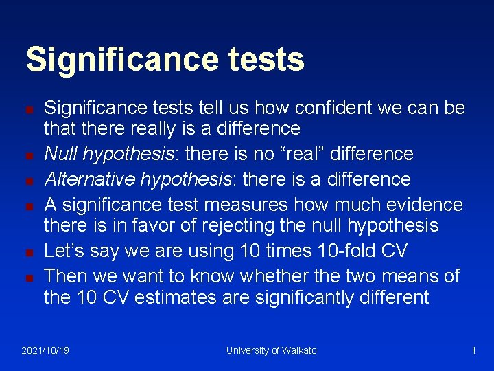
Significance tests n n n Significance tests tell us how confident we can be that there really is a difference Null hypothesis: there is no “real” difference Alternative hypothesis: there is a difference A significance test measures how much evidence there is in favor of rejecting the null hypothesis Let’s say we are using 10 times 10 -fold CV Then we want to know whether the two means of the 10 CV estimates are significantly different 2021/10/19 University of Waikato 1

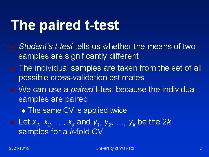
The paired t-test n n n Student’s t-test tells us whether the means of two samples are significantly different The individual samples are taken from the set of all possible cross-validation estimates We can use a paired t-test because the individual samples are paired u n The same CV is applied twice Let x 1, x 2, …, xk and y 1, y 2, …, yk be the 2 k samples for a k-fold CV 2021/10/19 University of Waikato 2

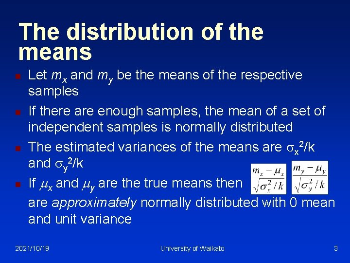
The distribution of the means n n Let mx and my be the means of the respective samples If there are enough samples, the mean of a set of independent samples is normally distributed The estimated variances of the means are x 2/k and y 2/k If x and y are the true means then are approximately normally distributed with 0 mean and unit variance 2021/10/19 University of Waikato 3

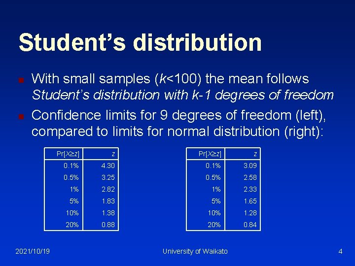
Student’s distribution n n With small samples (k<100) the mean follows Student’s distribution with k-1 degrees of freedom Confidence limits for 9 degrees of freedom (left), compared to limits for normal distribution (right): 2021/10/19 Pr[X z] z 0. 1% 4. 30 0. 1% 3. 09 0. 5% 3. 25 0. 5% 2. 58 1% 2. 82 1% 2. 33 5% 1. 83 5% 1. 65 10% 1. 38 10% 1. 28 20% 0. 84 University of Waikato 4

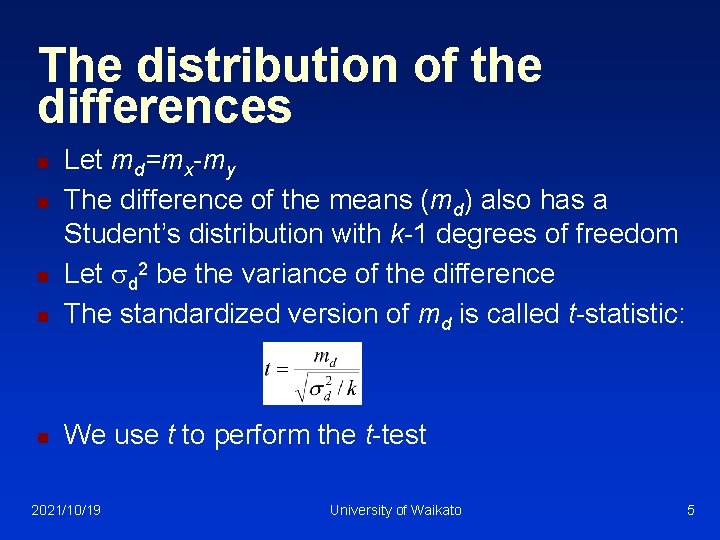
The distribution of the differences n Let md=mx-my The difference of the means (md) also has a Student’s distribution with k-1 degrees of freedom Let d 2 be the variance of the difference The standardized version of md is called t-statistic: n We use t to perform the t-test n n n 2021/10/19 University of Waikato 5

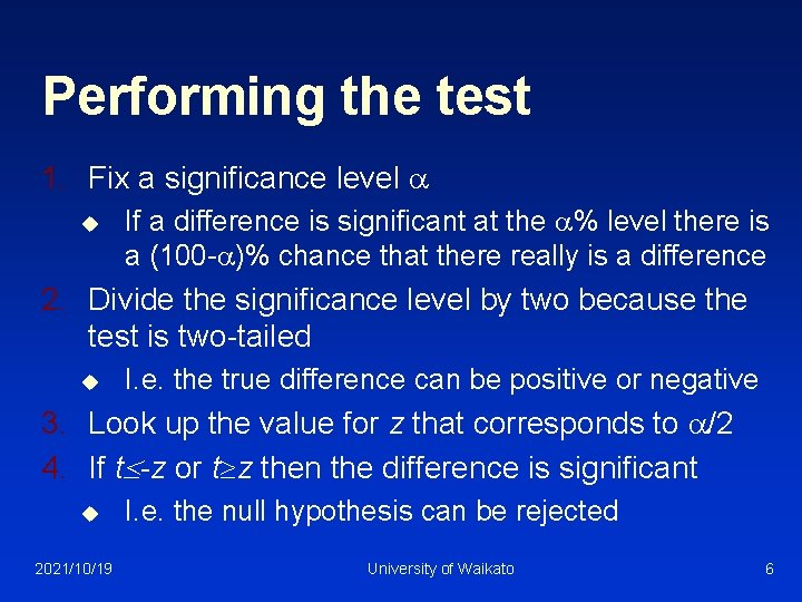
Performing the test 1. Fix a significance level u If a difference is significant at the % level there is a (100 - )% chance that there really is a difference 2. Divide the significance level by two because the test is two-tailed u I. e. the true difference can be positive or negative 3. Look up the value for z that corresponds to /2 4. If t -z or t z then the difference is significant u 2021/10/19 I. e. the null hypothesis can be rejected University of Waikato 6

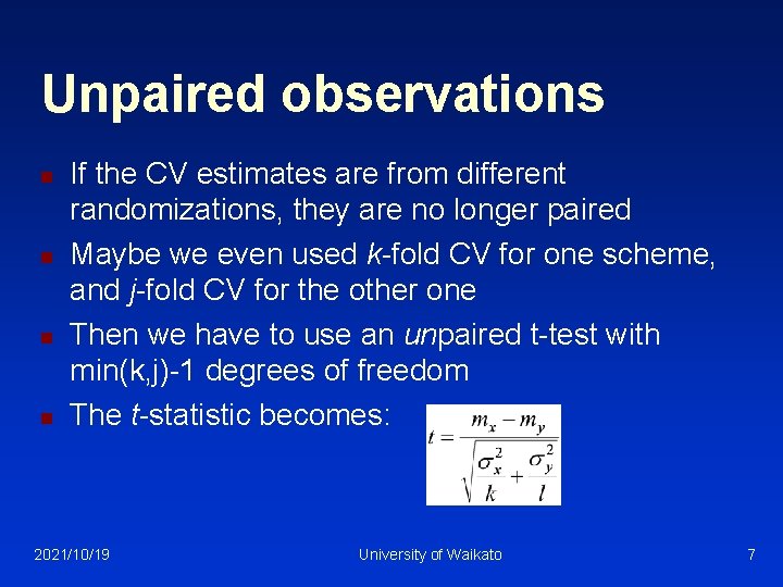
Unpaired observations n n If the CV estimates are from different randomizations, they are no longer paired Maybe we even used k-fold CV for one scheme, and j-fold CV for the other one Then we have to use an unpaired t-test with min(k, j)-1 degrees of freedom The t-statistic becomes: 2021/10/19 University of Waikato 7

A note on interpreting the result n n All our cross-validation estimates are based on the same dataset Hence the test only tells us whether a complete kfold CV for this dataset would show a difference u n Complete k-fold CV generates all possible partitions of the data into k folds and averages the results Ideally, we want a different dataset sample for each of the k-fold CV estimates used in the test to judge performance across different training sets 2021/10/19 University of Waikato 8

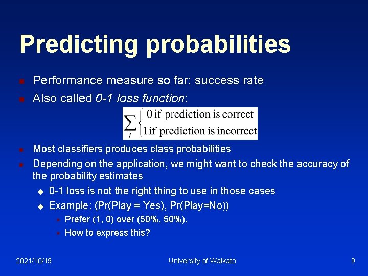
Predicting probabilities n n Performance measure so far: success rate Also called 0 -1 loss function: Most classifiers produces class probabilities Depending on the application, we might want to check the accuracy of the probability estimates u 0 -1 loss is not the right thing to use in those cases u Example: (Pr(Play = Yes), Pr(Play=No)) « « 2021/10/19 Prefer (1, 0) over (50%, 50%). How to express this? University of Waikato 9

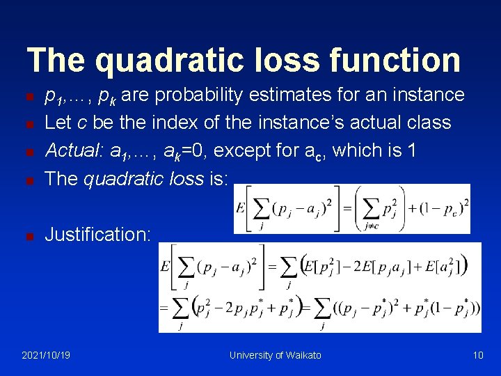
The quadratic loss function n p 1, …, pk are probability estimates for an instance Let c be the index of the instance’s actual class Actual: a 1, …, ak=0, except for ac, which is 1 The quadratic loss is: n Justification: n n n 2021/10/19 University of Waikato 10

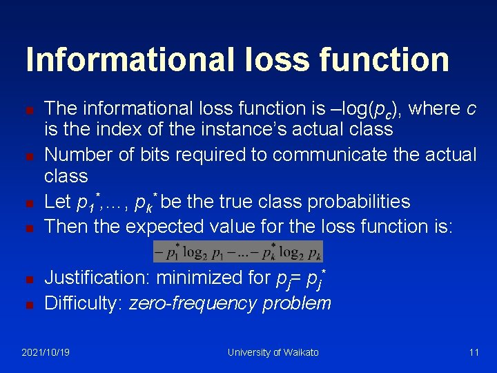
Informational loss function n n n The informational loss function is –log(pc), where c is the index of the instance’s actual class Number of bits required to communicate the actual class Let p 1*, …, pk* be the true class probabilities Then the expected value for the loss function is: Justification: minimized for pj= pj* Difficulty: zero-frequency problem 2021/10/19 University of Waikato 11

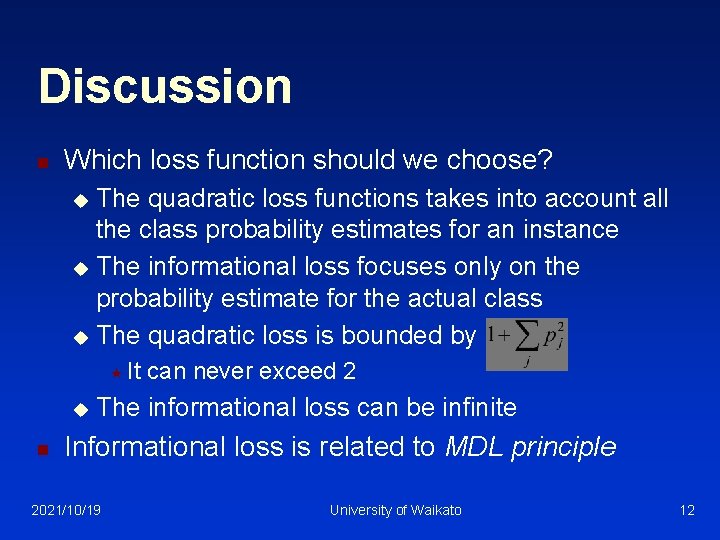
Discussion n Which loss function should we choose? The quadratic loss functions takes into account all the class probability estimates for an instance u The informational loss focuses only on the probability estimate for the actual class u The quadratic loss is bounded by u « It u n can never exceed 2 The informational loss can be infinite Informational loss is related to MDL principle 2021/10/19 University of Waikato 12

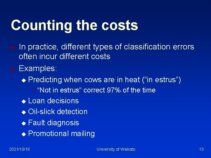
Counting the costs n n In practice, different types of classification errors often incur different costs Examples: u Predicting when cows are in heat (“in estrus”) « “Not in estrus” correct 97% of the time Loan decisions u Oil-slick detection u Fault diagnosis u Promotional mailing u 2021/10/19 University of Waikato 13

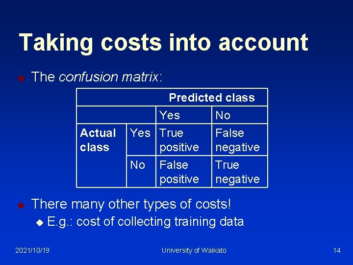
Taking costs into account n The confusion matrix: Actual class Predicted class Yes No Yes True False positive negative No n False positive True negative There many other types of costs! u E. g. : cost of collecting training data 2021/10/19 University of Waikato 14

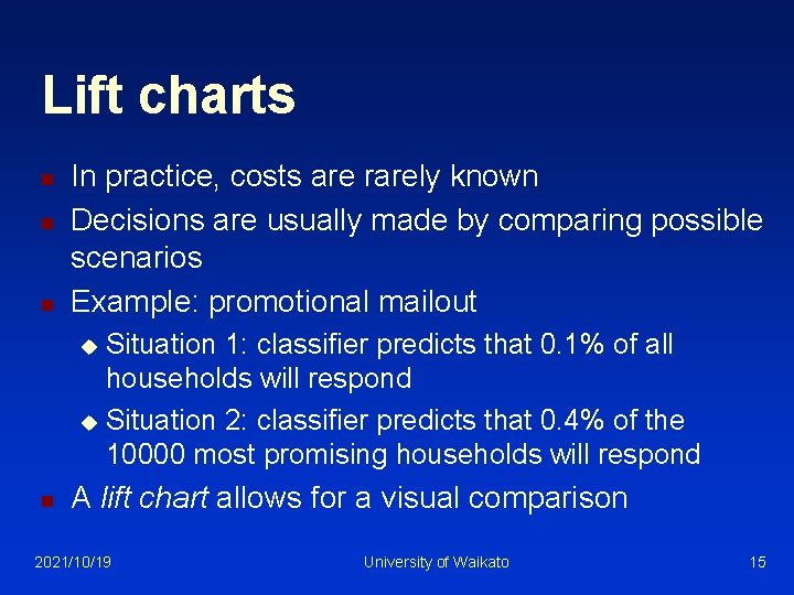
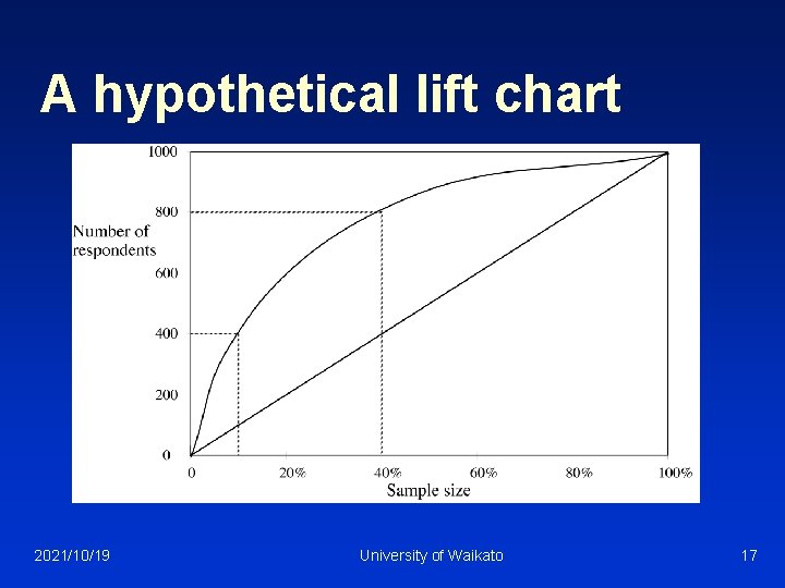
Lift charts n n n In practice, costs are rarely known Decisions are usually made by comparing possible scenarios Example: promotional mailout Situation 1: classifier predicts that 0. 1% of all households will respond u Situation 2: classifier predicts that 0. 4% of the 10000 most promising households will respond u n A lift chart allows for a visual comparison 2021/10/19 University of Waikato 15

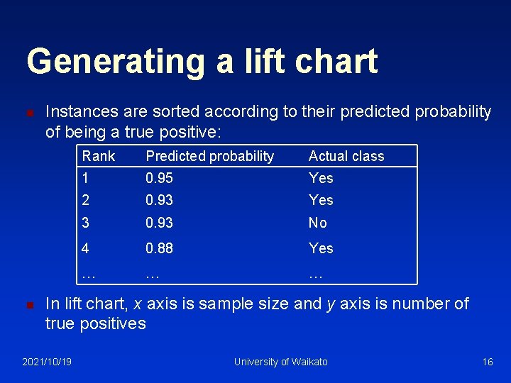
Generating a lift chart n n Instances are sorted according to their predicted probability of being a true positive: Rank Predicted probability Actual class 1 0. 95 Yes 2 0. 93 Yes 3 0. 93 No 4 0. 88 Yes … … … In lift chart, x axis is sample size and y axis is number of true positives 2021/10/19 University of Waikato 16

A hypothetical lift chart 2021/10/19 University of Waikato 17

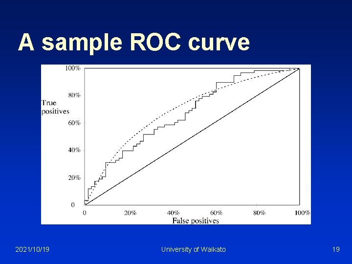
ROC curves n ROC curves are similar to lift charts “ROC” stands for “receiver operating characteristic” u Used in signal detection to show tradeoff between hit rate and false alarm rate over noisy channel u n Differences to lift chart: y axis shows percentage of true positives in sample (rather than absolute number) u x axis shows percentage of false positives in sample (rather than sample size) u 2021/10/19 University of Waikato 18

A sample ROC curve 2021/10/19 University of Waikato 19

Cross-validation and ROC curves n Simple method of getting a ROC curve using cross -validation: Collect probabilities for instances in test folds u Sort instances according to probabilities u n n This method is implemented in WEKA However, this is just one possibility u The method described in the book generates an ROC curve for each fold and averages them 2021/10/19 University of Waikato 20

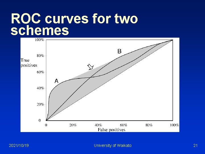
ROC curves for two schemes 2021/10/19 University of Waikato 21

The convex hull n n Given two learning schemes we can achieve any point on the convex hull! TP and FP rates for scheme 1: t 1 and f 1 TP and FP rates for scheme 2: t 2 and f 2 If scheme 1 is used to predict 100 q% of the cases and scheme 2 for the rest, then we get: TP rate for combined scheme: q t 1+(1 -q) t 2 u FP rate for combined scheme: q f 2+(1 -q) f 2 u 2021/10/19 University of Waikato 22

Cost-sensitive learning n Most learning schemes do not perform costsensitive learning They generate the same classifier no matter what costs are assigned to the different classes u Example: standard decision tree learner u n Simple methods for cost-sensitive learning: Resampling of instances according to costs u Weighting of instances according to costs u n Some schemes are inherently cost-sensitive, e. g. naïve Bayes 2021/10/19 University of Waikato 23

Measures in information retrieval n n n Percentage of retrieved documents that are relevant: precision=TP/TP+FP Percentage of relevant documents that are returned: recall =TP/TP+FN Precision/recall curves have hyperbolic shape Summary measures: average precision at 20%, 50% and 80% recall (three-point average recall) F-measure=(2 recall precision)/(recall+precision) 2021/10/19 University of Waikato 24

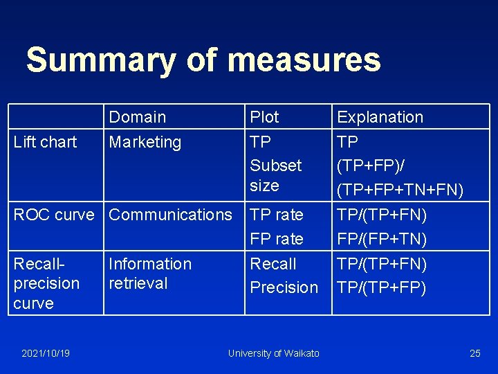
Summary of measures Lift chart Domain Marketing ROC curve Communications Recallprecision curve 2021/10/19 Information retrieval Plot TP Subset size Explanation TP (TP+FP)/ (TP+FP+TN+FN) TP rate FP rate Recall Precision TP/(TP+FN) FP/(FP+TN) TP/(TP+FP) University of Waikato 25

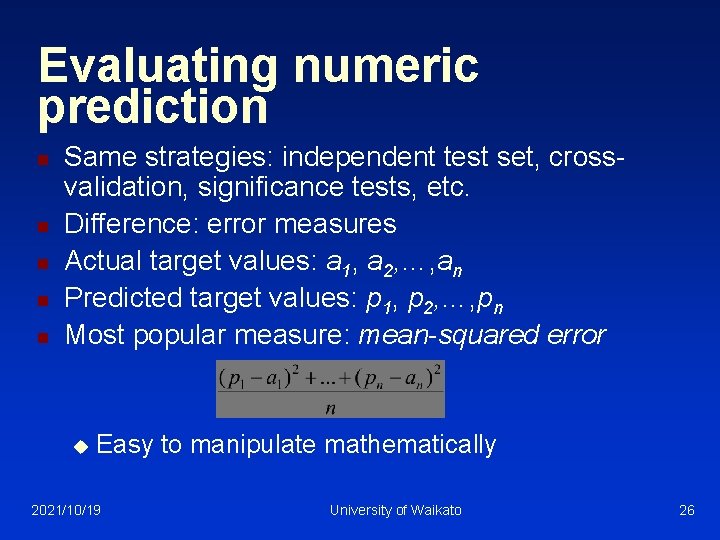
Evaluating numeric prediction n n Same strategies: independent test set, crossvalidation, significance tests, etc. Difference: error measures Actual target values: a 1, a 2, …, an Predicted target values: p 1, p 2, …, pn Most popular measure: mean-squared error u Easy to manipulate mathematically 2021/10/19 University of Waikato 26

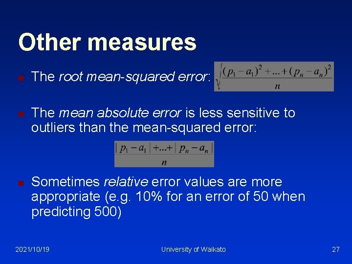
Other measures n n n The root mean-squared error: The mean absolute error is less sensitive to outliers than the mean-squared error: Sometimes relative error values are more appropriate (e. g. 10% for an error of 50 when predicting 500) 2021/10/19 University of Waikato 27

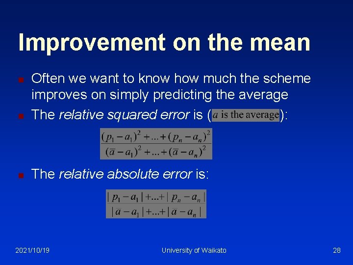
Improvement on the mean n Often we want to know how much the scheme improves on simply predicting the average The relative squared error is ( ): n The relative absolute error is: n 2021/10/19 University of Waikato 28

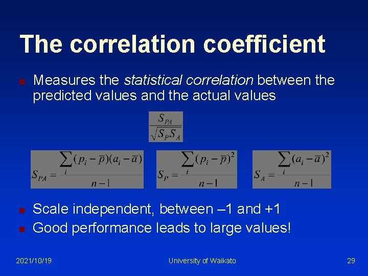
The correlation coefficient n n n Measures the statistical correlation between the predicted values and the actual values Scale independent, between – 1 and +1 Good performance leads to large values! 2021/10/19 University of Waikato 29

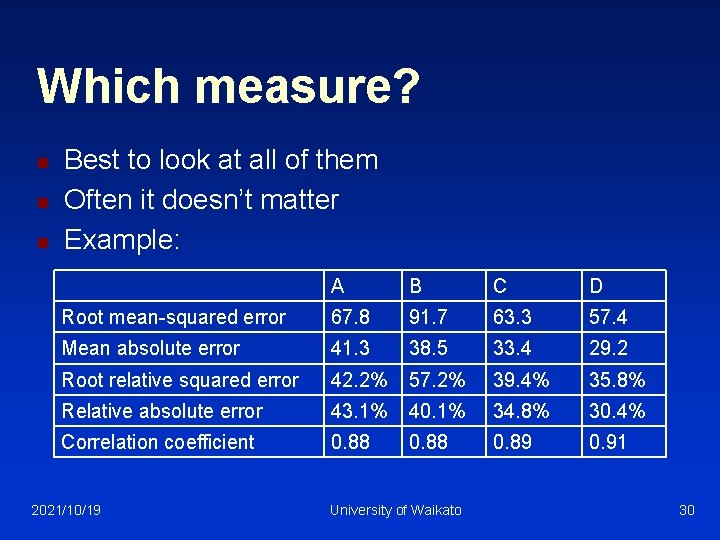
Which measure? n n n Best to look at all of them Often it doesn’t matter Example: A B C D Root mean-squared error 67. 8 91. 7 63. 3 57. 4 Mean absolute error 41. 3 38. 5 33. 4 29. 2 Root relative squared error 42. 2% 57. 2% 39. 4% 35. 8% Relative absolute error 43. 1% 40. 1% 34. 8% 30. 4% Correlation coefficient 0. 88 0. 89 0. 91 2021/10/19 University of Waikato 30

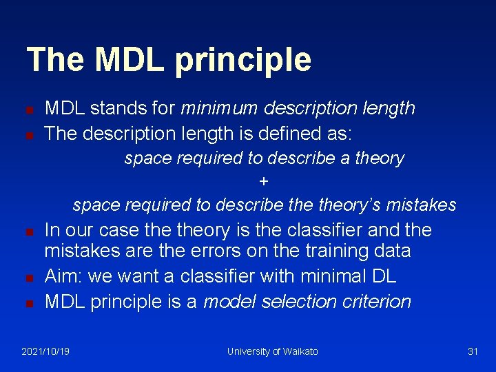
The MDL principle n n MDL stands for minimum description length The description length is defined as: space required to describe a theory + space required to describe theory’s mistakes n n n In our case theory is the classifier and the mistakes are the errors on the training data Aim: we want a classifier with minimal DL MDL principle is a model selection criterion 2021/10/19 University of Waikato 31

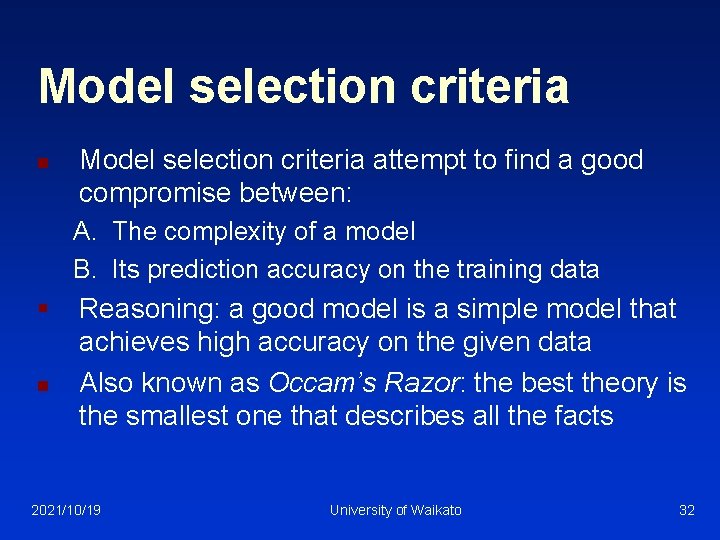
Model selection criteria n Model selection criteria attempt to find a good compromise between: A. The complexity of a model B. Its prediction accuracy on the training data § n Reasoning: a good model is a simple model that achieves high accuracy on the given data Also known as Occam’s Razor: the best theory is the smallest one that describes all the facts 2021/10/19 University of Waikato 32

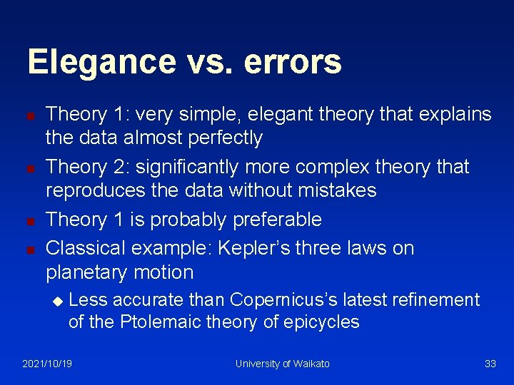
Elegance vs. errors n n Theory 1: very simple, elegant theory that explains the data almost perfectly Theory 2: significantly more complex theory that reproduces the data without mistakes Theory 1 is probably preferable Classical example: Kepler’s three laws on planetary motion u Less accurate than Copernicus’s latest refinement of the Ptolemaic theory of epicycles 2021/10/19 University of Waikato 33

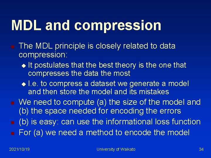
MDL and compression n The MDL principle is closely related to data compression: It postulates that the best theory is the one that compresses the data the most u I. e. to compress a dataset we generate a model and then store the model and its mistakes u n n n We need to compute (a) the size of the model and (b) the space needed for encoding the errors (b) is easy: can use the informational loss function For (a) we need a method to encode the model 2021/10/19 University of Waikato 34

DL and Bayes’s theorem n n L[T]=“length” of theory L[E|T]=training set encoded wrt. theory Description length= L[T] + L[E|T] Bayes’s theorem gives us the a posteriori probability of a theory given the data: constant n Equivalent to: 2021/10/19 University of Waikato 35

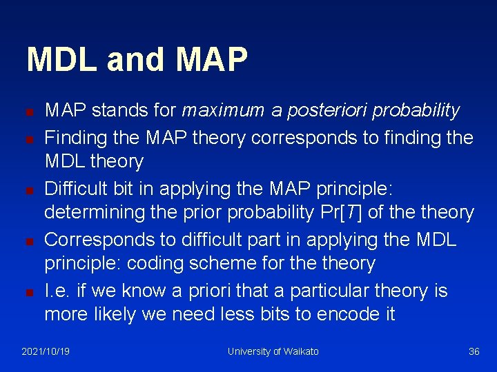
MDL and MAP n n n MAP stands for maximum a posteriori probability Finding the MAP theory corresponds to finding the MDL theory Difficult bit in applying the MAP principle: determining the prior probability Pr[T] of theory Corresponds to difficult part in applying the MDL principle: coding scheme for theory I. e. if we know a priori that a particular theory is more likely we need less bits to encode it 2021/10/19 University of Waikato 36

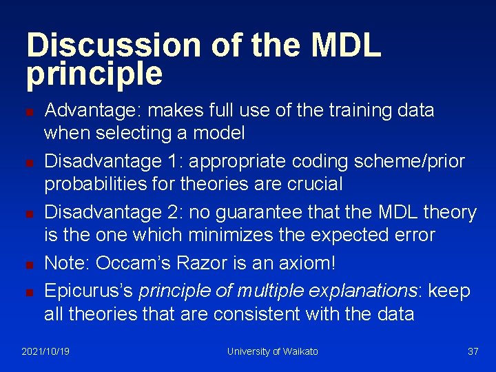
Discussion of the MDL principle n n n Advantage: makes full use of the training data when selecting a model Disadvantage 1: appropriate coding scheme/prior probabilities for theories are crucial Disadvantage 2: no guarantee that the MDL theory is the one which minimizes the expected error Note: Occam’s Razor is an axiom! Epicurus’s principle of multiple explanations: keep all theories that are consistent with the data 2021/10/19 University of Waikato 37

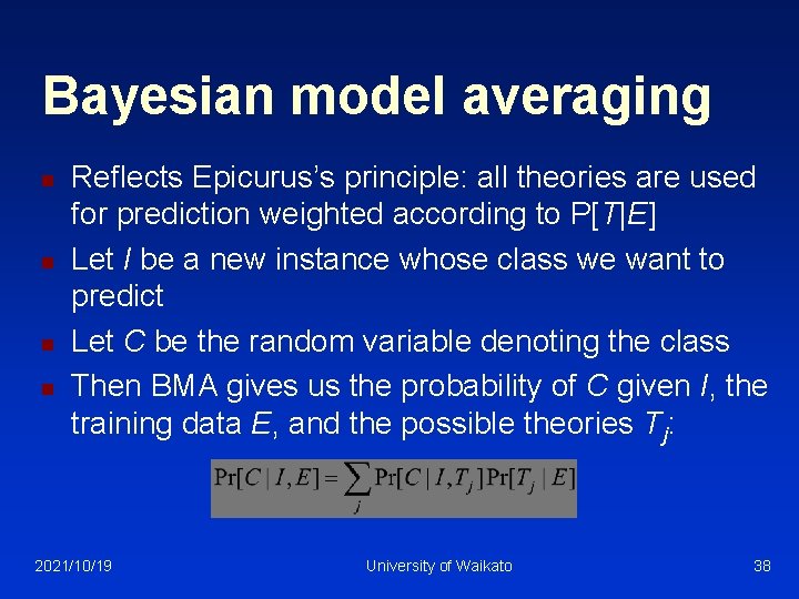
Bayesian model averaging n n Reflects Epicurus’s principle: all theories are used for prediction weighted according to P[T|E] Let I be a new instance whose class we want to predict Let C be the random variable denoting the class Then BMA gives us the probability of C given I, the training data E, and the possible theories Tj: 2021/10/19 University of Waikato 38

MDL and clustering n n DL of theory: DL needed for encoding the clusters (e. g. cluster centers) DL of data given theory: need to encode cluster membership and position relative to cluster (e. g. distance to cluster center) Works if coding scheme needs less code space for small numbers than for large ones With nominal attributes, we need to communicate probability distributions for each cluster 2021/10/19 University of Waikato 39