Significance Testing Univariate Significance Tests Purposes of NHST

Significance Testing & Univariate Significance Tests • Purposes of NHST • Process of Null Hypothesis Significance Testing • Univariate Significance Tests

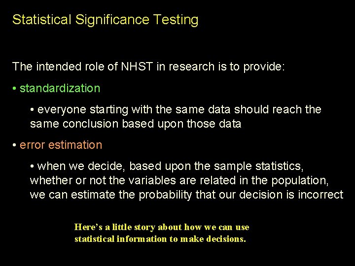
Statistical Significance Testing The intended role of NHST in research is to provide: • standardization • everyone starting with the same data should reach the same conclusion based upon those data • error estimation • when we decide, based upon the sample statistics, whether or not the variables are related in the population, we can estimate the probability that our decision is incorrect Here’s a little story about how we can use statistical information to make decisions.

Just imagine… You’re at the first of 12 home games of your favorite team. You’re sitting in the reserved seat you’ll enjoy all season. Just before half-time, the person in the seat next to you says, “Hey, how about if before each halftime we flip a coin to see who buys munchies? Heads you buy, tails I’ll buy. I have this official team coin we can use all 12 times. Hey, what do you know, its heads. I’ll have some popcorn, a hot dog, a candy bar and a drink! Want help carrying that? ” You don’t think much of it because you know that it’s a 50 -50 thing -- just your turn to lose! The next game the coin lands heads again, and you buy your “new friend” hot chocolate, a Polish Dog, fries and some peanuts. Still no worries, a couple in a row as pretty likely. The next game you buy him a couple of Runza’s, some cotton candy and an orange drink. Finally, you’re starting to get suspicious! Before the next game you have a chance to talk with a friend or yours who has had a statistics course. You ask your friend, “I’ve bought snacks all three times, which could happen if the coin were fair, but I don’t know how many more times I can expect to feed this person before the season is up. How do I know whether I should “confront” them or just keep politely buying snacks? ”

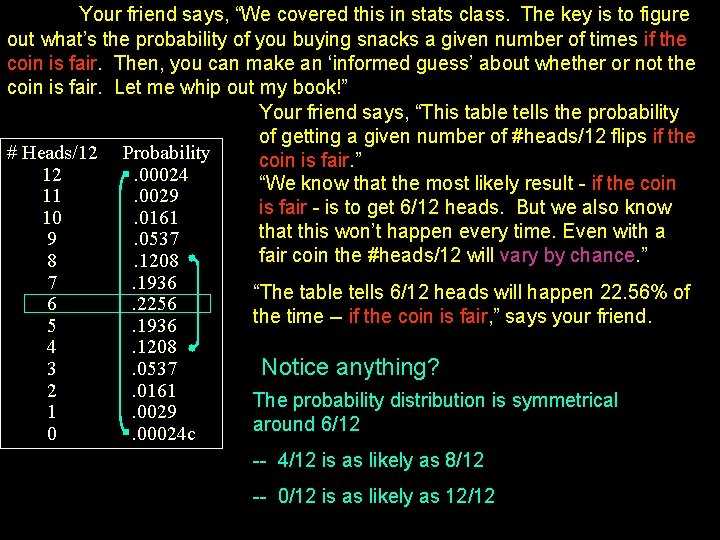
Your friend says, “We covered this in stats class. The key is to figure out what’s the probability of you buying snacks a given number of times if the coin is fair. Then, you can make an ‘informed guess’ about whether or not the coin is fair. Let me whip out my book!” Your friend says, “This table tells the probability of getting a given number of #heads/12 flips if the # Heads/12 Probability coin is fair. ” 12. 00024 “We know that the most likely result - if the coin 11. 0029 is fair - is to get 6/12 heads. But we also know 10. 0161 that this won’t happen every time. Even with a 9. 0537 fair coin the #heads/12 will vary by chance. ” 8. 1208 7. 1936 “The table tells 6/12 heads will happen 22. 56% of 6. 2256 the time -- if the coin is fair, ” says your friend. 5. 1936 4. 1208 Notice anything? 3. 0537 2. 0161 The probability distribution is symmetrical 1. 0029 around 6/12 0. 00024 c -- 4/12 is as likely as 8/12 -- 0/12 is as likely as 12/12

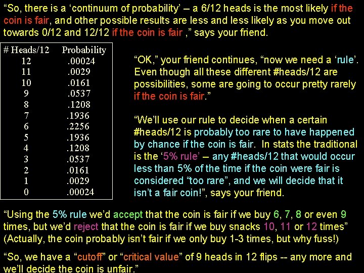
“So, there is a ‘continuum of probability’ -- a 6/12 heads is the most likely if the coin is fair, and other possible results are less and less likely as you move out towards 0/12 and 12/12 if the coin is fair , ” says your friend. # Heads/12 12 11 10 9 8 7 6 5 4 3 2 1 0 Probability. 00024. 0029. 0161. 0537. 1208. 1936. 2256. 1936. 1208. 0537. 0161. 0029. 00024 “OK, ” your friend continues, “now we need a ‘rule’. Even though all these different #heads/12 are possibilities, some are going to occur pretty rarely if the coin is fair. ” “We’ll use our rule to decide when a certain #heads/12 is probably too rare to have happened by chance if the coin is fair. In stats the traditional is the ‘ 5% rule’ -- any #heads/12 that would occur less than 5% of the time if the coin were fair is considered “too rare”, and we will decide that it isn’t a fair coin!”, says your friend. “Using the 5% rule we’d accept that the coin is fair if we buy 6, 7, 8 or even 9 times, but we’d reject that the coin is fair if we buy snacks 10, 11 or 12 times” (Actually, the coin probably isn’t fair if we only buy 1 -3 times, but why fuss!) “So, we have a “cutoff” or “critical value” of 9 heads in 12 flips -- any more and we’ll decide the coin is unfair. ”

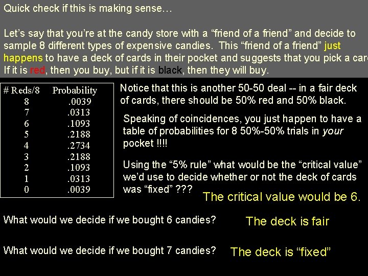
Quick check if this is making sense… Let’s say that you’re at the candy store with a “friend of a friend” and decide to sample 8 different types of expensive candies. This “friend of a friend” just happens to have a deck of cards in their pocket and suggests that you pick a card If it is red, then you buy, but if it is black, then they will buy. # Reds/8 8 7 6 5 4 3 2 1 0 Probability. 0039. 0313. 1093. 2188. 2734. 2188. 1093. 0313. 0039 Notice that this is another 50 -50 deal -- in a fair deck of cards, there should be 50% red and 50% black. Speaking of coincidences, you just happen to have a table of probabilities for 8 50%-50% trials in your pocket !!!! Using the “ 5% rule” what would be the “critical value” we’d use to decide whether or not the deck of cards was “fixed” ? ? ? The critical value would be 6. What would we decide if we bought 6 candies? The deck is fair What would we decide if we bought 7 candies? The deck is “fixed”

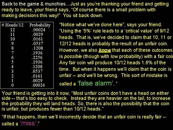
Back to the game & munchies…Just as you’re thanking your friend and getting ready to leave, your friend says, “Of course there is a small problem with making decisions this way!” You sit back down. # Heads/12 12 11 10 9 8 7 6 5 4 3 2 1 0 Probability. 00024. 0029. 0161. 0537. 1208. 1936. 2256. 1936. 1208. 0537. 0161. 0029. 00024 “Notice what we’ve done here”, says your friend. “Using the ‘ 5%’ rule leads to a ‘critical value’ of 9/12 heads. That is, we’ve decided to claim that 10, 11 or 12/12 heads is probably the result of an unfair coin. However, we also know that each of these outcomes is possible (though with low probability) with a fair coin Any fair coin will produce 10/12 heads 1. 6% of the time. But when it happens we’ll claim that the coin is unfair -- and we’ll be wrong. This sort of mistake is called a ‘false alarm’. ” Your friend is getting into it now, “Most unfair coins don’t have a head on either side -- that’s too easy to check. Instead they are heavier on the tail, to increase the probability they will land heads. So, there is also the possibility that the coin is unfair, but produces fewer than 10/12 heads. ” “If that happens, then we’ll incorrectly decide that an unfair coin is really fair -called a ‘miss’. ”

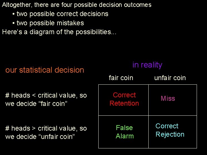
Altogether, there are four possible decision outcomes • two possible correct decisions • two possible mistakes Here’s a diagram of the possibilities. . . our statistical decision in reality fair coin # heads < critical value, so we decide “fair coin” Correct Retention # heads > critical value, so we decide “unfair coin” False Alarm unfair coin Miss Correct Rejection

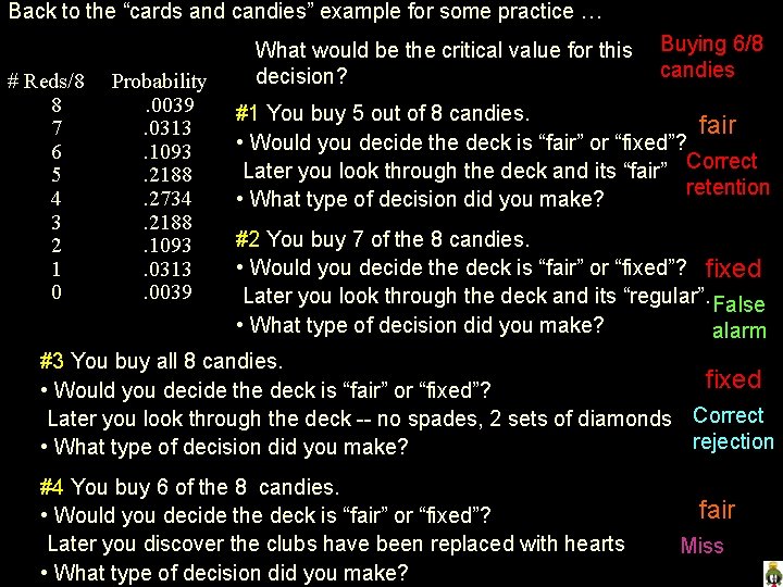
Back to the “cards and candies” example for some practice … # Reds/8 8 7 6 5 4 3 2 1 0 Probability. 0039. 0313. 1093. 2188. 2734. 2188. 1093. 0313. 0039 What would be the critical value for this decision? Buying 6/8 candies #1 You buy 5 out of 8 candies. fair • Would you decide the deck is “fair” or “fixed”? Later you look through the deck and its “fair” Correct retention • What type of decision did you make? #2 You buy 7 of the 8 candies. • Would you decide the deck is “fair” or “fixed”? fixed Later you look through the deck and its “regular”. False • What type of decision did you make? alarm #3 You buy all 8 candies. fixed • Would you decide the deck is “fair” or “fixed”? Later you look through the deck -- no spades, 2 sets of diamonds Correct rejection • What type of decision did you make? #4 You buy 6 of the 8 candies. • Would you decide the deck is “fair” or “fixed”? Later you discover the clubs have been replaced with hearts • What type of decision did you make? fair Miss

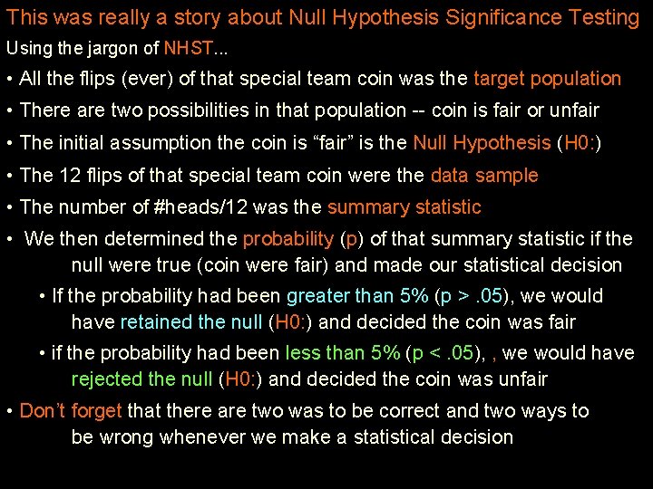
This was really a story about Null Hypothesis Significance Testing Using the jargon of NHST. . . • All the flips (ever) of that special team coin was the target population • There are two possibilities in that population -- coin is fair or unfair • The initial assumption the coin is “fair” is the Null Hypothesis (H 0: ) • The 12 flips of that special team coin were the data sample • The number of #heads/12 was the summary statistic • We then determined the probability (p) of that summary statistic if the null were true (coin were fair) and made our statistical decision • If the probability had been greater than 5% (p >. 05), we would have retained the null (H 0: ) and decided the coin was fair • if the probability had been less than 5% (p <. 05), , we would have rejected the null (H 0: ) and decided the coin was unfair • Don’t forget that there are two was to be correct and two ways to be wrong whenever we make a statistical decision

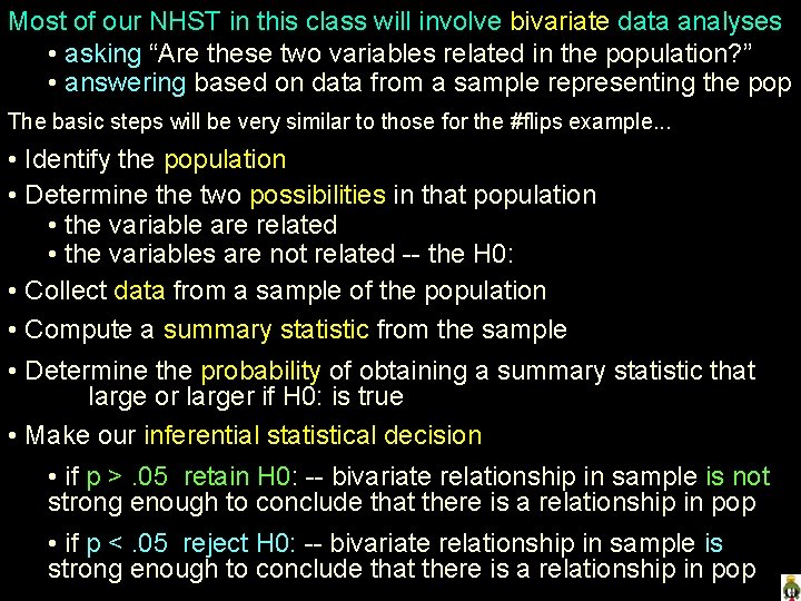
Most of our NHST in this class will involve bivariate data analyses • asking “Are these two variables related in the population? ” • answering based on data from a sample representing the pop The basic steps will be very similar to those for the #flips example. . . • Identify the population • Determine the two possibilities in that population • the variable are related • the variables are not related -- the H 0: • Collect data from a sample of the population • Compute a summary statistic from the sample • Determine the probability of obtaining a summary statistic that large or larger if H 0: is true • Make our inferential statistical decision • if p >. 05 retain H 0: -- bivariate relationship in sample is not strong enough to conclude that there is a relationship in pop • if p <. 05 reject H 0: -- bivariate relationship in sample is strong enough to conclude that there is a relationship in pop

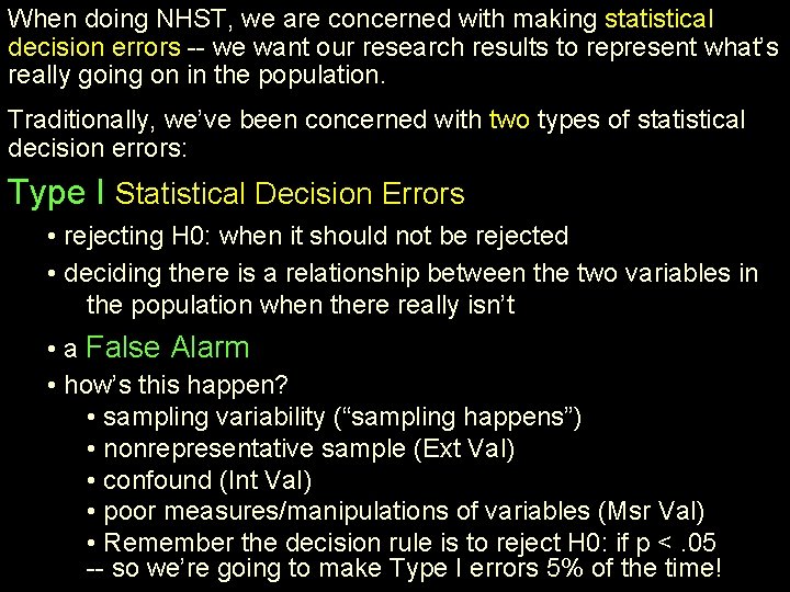
When doing NHST, we are concerned with making statistical decision errors -- we want our research results to represent what’s really going on in the population. Traditionally, we’ve been concerned with two types of statistical decision errors: Type I Statistical Decision Errors • rejecting H 0: when it should not be rejected • deciding there is a relationship between the two variables in the population when there really isn’t • a False Alarm • how’s this happen? • sampling variability (“sampling happens”) • nonrepresentative sample (Ext Val) • confound (Int Val) • poor measures/manipulations of variables (Msr Val) • Remember the decision rule is to reject H 0: if p <. 05 -- so we’re going to make Type I errors 5% of the time!

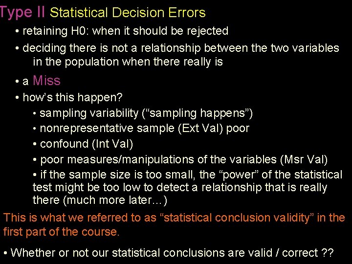
Type II Statistical Decision Errors • retaining H 0: when it should be rejected • deciding there is not a relationship between the two variables in the population when there really is • a Miss • how’s this happen? • sampling variability (“sampling happens”) • nonrepresentative sample (Ext Val) poor • confound (Int Val) • poor measures/manipulations of the variables (Msr Val) • if the sample size is too small, the “power” of the statistical test might be too low to detect a relationship that is really there (much more later…) This is what we referred to as “statistical conclusion validity” in the first part of the course. • Whether or not our statistical conclusions are valid / correct ? ?

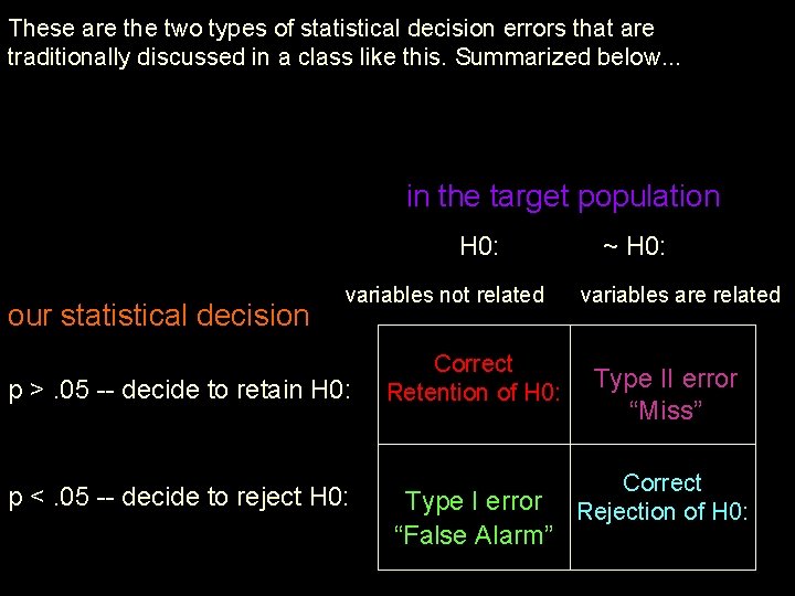
These are the two types of statistical decision errors that are traditionally discussed in a class like this. Summarized below. . . in the target population H 0: our statistical decision variables not related p >. 05 -- decide to retain H 0: p <. 05 -- decide to reject H 0: Correct Retention of H 0: Type I error “False Alarm” ~ H 0: variables are related Type II error “Miss” Correct Rejection of H 0:

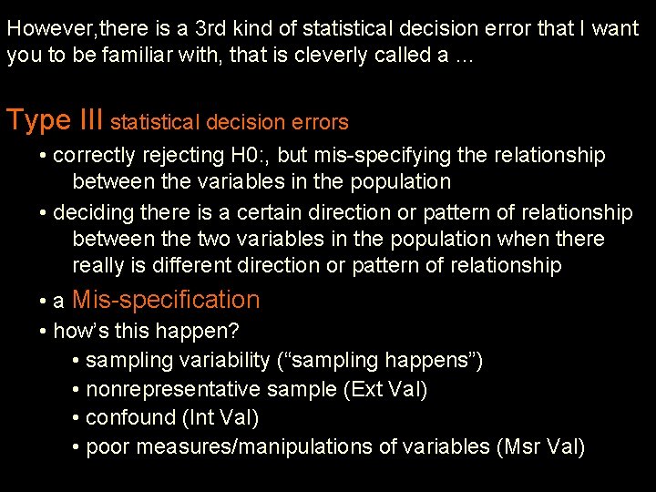
However, there is a 3 rd kind of statistical decision error that I want you to be familiar with, that is cleverly called a … Type III statistical decision errors • correctly rejecting H 0: , but mis-specifying the relationship between the variables in the population • deciding there is a certain direction or pattern of relationship between the two variables in the population when there really is different direction or pattern of relationship • a Mis-specification • how’s this happen? • sampling variability (“sampling happens”) • nonrepresentative sample (Ext Val) • confound (Int Val) • poor measures/manipulations of variables (Msr Val)

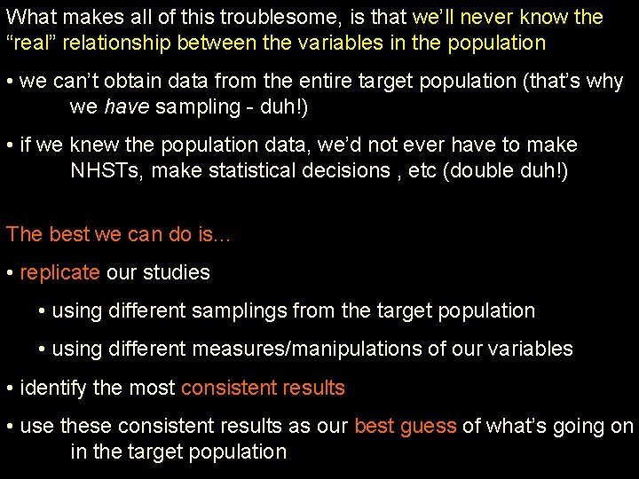
What makes all of this troublesome, is that we’ll never know the “real” relationship between the variables in the population • we can’t obtain data from the entire target population (that’s why we have sampling - duh!) • if we knew the population data, we’d not ever have to make NHSTs, make statistical decisions , etc (double duh!) The best we can do is. . . • replicate our studies • using different samplings from the target population • using different measures/manipulations of our variables • identify the most consistent results • use these consistent results as our best guess of what’s going on in the target population

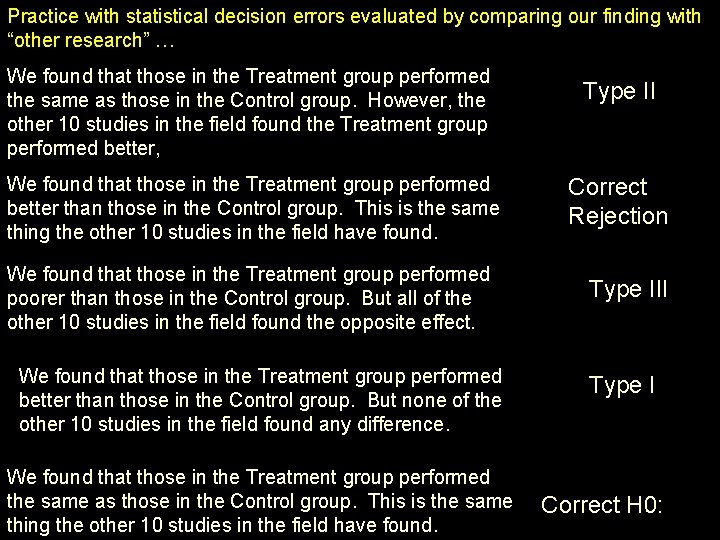
Practice with statistical decision errors evaluated by comparing our finding with “other research” … We found that those in the Treatment group performed the same as those in the Control group. However, the other 10 studies in the field found the Treatment group performed better, We found that those in the Treatment group performed better than those in the Control group. This is the same thing the other 10 studies in the field have found. We found that those in the Treatment group performed poorer than those in the Control group. But all of the other 10 studies in the field found the opposite effect. We found that those in the Treatment group performed better than those in the Control group. But none of the other 10 studies in the field found any difference. We found that those in the Treatment group performed the same as those in the Control group. This is the same thing the other 10 studies in the field have found. Type II Correct Rejection Type III Type I Correct H 0:

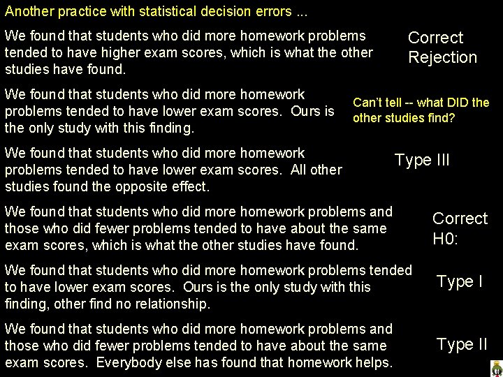
Another practice with statistical decision errors. . . We found that students who did more homework problems tended to have higher exam scores, which is what the other studies have found. We found that students who did more homework problems tended to have lower exam scores. Ours is the only study with this finding. Correct Rejection Can’t tell -- what DID the other studies find? We found that students who did more homework problems tended to have lower exam scores. All other studies found the opposite effect. Type III We found that students who did more homework problems and those who did fewer problems tended to have about the same exam scores, which is what the other studies have found. Correct H 0: We found that students who did more homework problems tended to have lower exam scores. Ours is the only study with this finding, other find no relationship. Type I We found that students who did more homework problems and those who did fewer problems tended to have about the same exam scores. Everybody else has found that homework helps. Type II

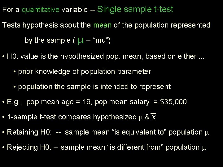
For a quantitative variable -- Single sample t-test Tests hypothesis about the mean of the population represented by the sample ( -- “mu”) • H 0: value is the hypothesized pop. mean, based on either. . . • prior knowledge of population parameter • population the sample is intended to represent • E. g. , pop mean age = 19, pop mean salary = $35, 000 • 1 -sample t-test compares hypothesized & x • Retaining H 0: -- sample mean “is equivalent to” population • Rejecting H 0: -- sample mean “is different from” population

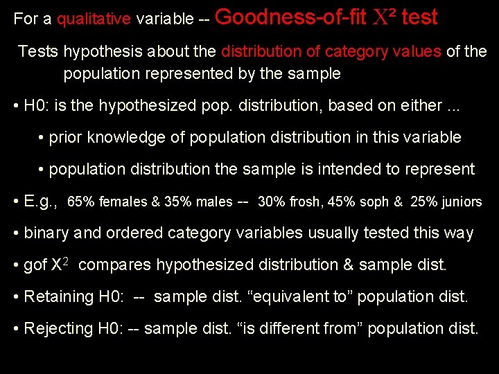
For a qualitative variable -- Goodness-of-fit ² test Tests hypothesis about the distribution of category values of the population represented by the sample • H 0: is the hypothesized pop. distribution, based on either. . . • prior knowledge of population distribution in this variable • population distribution the sample is intended to represent • E. g. , 65% females & 35% males -- 30% frosh, 45% soph & 25% juniors • binary and ordered category variables usually tested this way • gof X 2 compares hypothesized distribution & sample dist. • Retaining H 0: -- sample dist. “equivalent to” population dist. • Rejecting H 0: -- sample dist. “is different from” population dist.

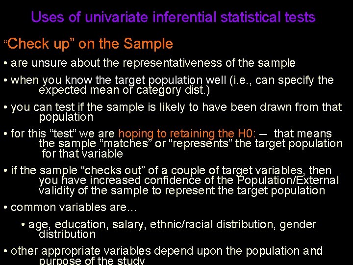
Uses of univariate inferential statistical tests “Check up” on the Sample • are unsure about the representativeness of the sample • when you know the target population well (i. e. , can specify the expected mean or category dist. ) • you can test if the sample is likely to have been drawn from that population • for this “test” we are hoping to retaining the H 0: -- that means the sample “matches” or “represents” the target population for that variable • if the sample “checks out” of a couple of target variables, then you have increased confidence of the Population/External validity of the sample to represent the target population • common variables are… • age, education, salary, ethnic/racial distribution, gender distribution • other appropriate variables depend upon the population and purpose of the study

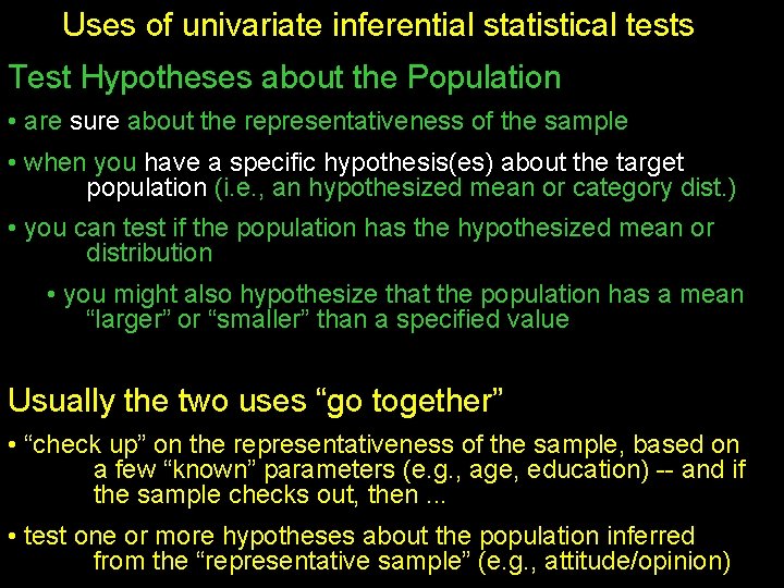
Uses of univariate inferential statistical tests Test Hypotheses about the Population • are sure about the representativeness of the sample • when you have a specific hypothesis(es) about the target population (i. e. , an hypothesized mean or category dist. ) • you can test if the population has the hypothesized mean or distribution • you might also hypothesize that the population has a mean “larger” or “smaller” than a specified value Usually the two uses “go together” • “check up” on the representativeness of the sample, based on a few “known” parameters (e. g. , age, education) -- and if the sample checks out, then. . . • test one or more hypotheses about the population inferred from the “representative sample” (e. g. , attitude/opinion)

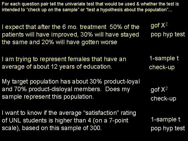
For each question pair tell the univariate test that would be used & whether the test is intended to “check up on the sample” or “test a hypothesis about the population”. . . I expect that after the 6 mo. treatment 50% of the patients will have improved, 30% will have stayed the same and 20% will have gotten worse gof X 2 pop hyp test I am trying to represent females that have an average of about 12 years of education. 1 -sample t check-up My target population has about 30% product-loyal and 70% product-disloyal members. Does my sample represent this population. gof X 2 check-up I want to know if the average “satisfaction” rating of UNL students is higher than 4 (on a 7 -point scale), based on this sample of 300. 1 -sample t pop hyp test