Shortest Paths Chapter 4 Acknowledgement I have used

Shortest Paths (Chapter 4)

Acknowledgement • I have used some slides from: http: //web. stanford. edu/class/archive/cs/cs 161. 1138/ http: //www. cs. sfu. ca/Course. Central/225/johnwill/schedule. html

• This chapter is about shortest paths. • The length of a path P (denoted |P|) in a graph is the number of edges in the graph. • A shortest path between u and v is a path P where |P| ≤ |P’| for any path P’ from u to v. • The distance between two nodes u and v in a graph is the length of the shortest path, denoted by d(u, v).

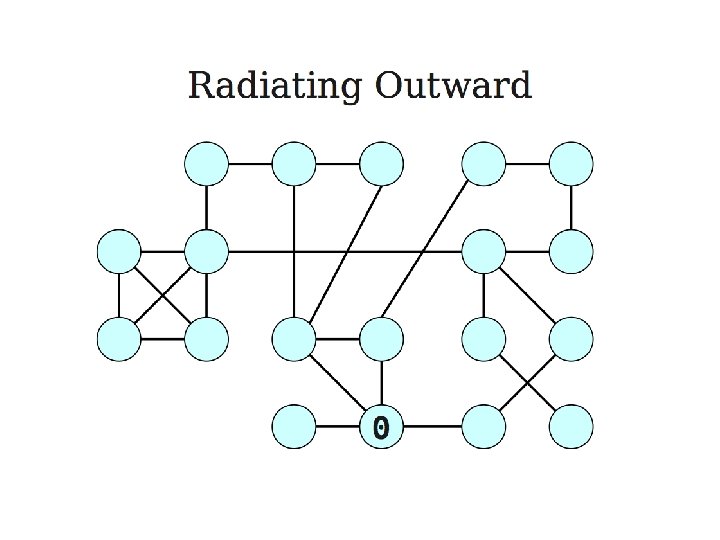
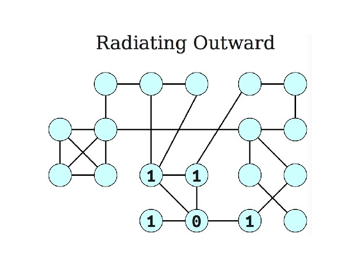
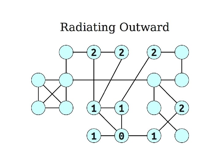
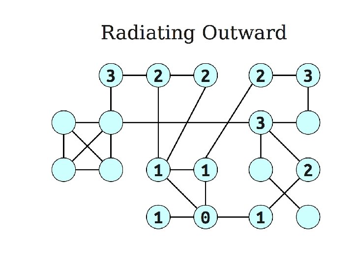
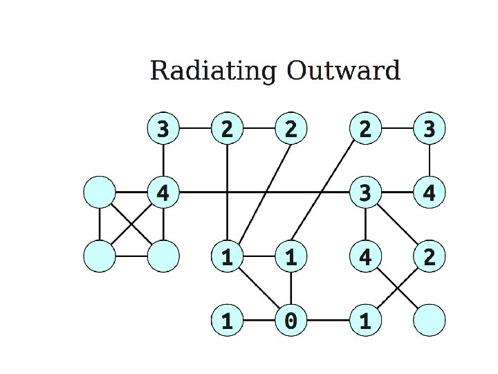
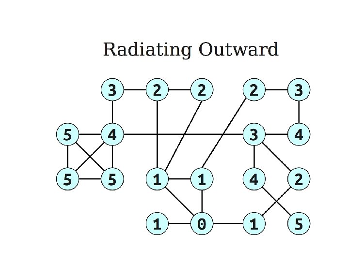
An application: Six degrees of separtion Source node The numbers on nodes indicate the distances of the nodes from the source node.

Source node

Source node Principle of optimality: If node A lies on the shortest path from the source node S to B then d (S, B) = d (S, A) + d ( A, B).

The shortest path problem • Input – A graph G=(V, E), which may be directed or undirected. – A start node s V. • Output – A table dist(v), where dist(v) = d(s, v) for any v V.

General Idea • Proceed outward from the source node s in ``layers’’. – The first layer is all nodes of distance 0. – The second layer is all nodes of distance 1. – The third layer is all nodes of distance 2. – etc. • This gives rise to breadth-first search.

Breadth-first search parent(v) = u

We keep only edges (thick ones) that correspond to parent field of some vertex.

Using the parent values • Using the parent values (π), how can we find a shortest path between s and v? v, π[v], π[π[v]], …, s

Correctness of BFS • We have developed the basic intuition behind BFS. • We need a proof that it faithfully executes the intuition. • Let S be the set of nodes whose distances from the source node s is known, i. e. dist[s, u] for all u in S is known. • Pick up a node v which is not an element of S, minimizing dist[s, v] + 1, where (u, v) is an edge of the graph and u is an element of S.

u v Lemma: Suppose we have shortest paths computed for nodes S ⊆ V, where s ∈ S. Consider a node v, not in S, where (u, v) ∈ E, u ∈ S, and the quantity dist(s, u) + 1 is minimized. Then dist(s, v) = dist(s, u) + 1.

Running time analysis • The total running time is O(|V|+|E|) (why? ) – Each vertex is put on the queue exactly once, when it is first encountered. – Therefore, there are 2|V| queue operations. – The rest of the work is done in the algorithm’s innermost loop. In this loop, each edge is being looked at exactly twice. – Over the course of execution, this loop takes O(|E|) time.

DFS vs. BFS • Input: • Idea: – A Graph G = (V, E) (directed or undirected) – No source vertex given! – Explore the edges of G to “discover” every vertex in V starting at the most current visited node – Search may be repeated from multiple sources • Output: – 2 timestamps on each vertex: pre[v], post[v] – DFS forest • O(|V|+|E|) BFS – A graph G = (V, E) (directed or undirected) – A source vertex s V – Explore the edges of G to “discover” every vertex reachable from s, taking the ones closest to s first • Output: – d[v] = distance (smallest # of edges, or shortest path) from s to v, for all v V – BFS tree • O(|V|+|E|) 21

Modified BFS Algorithm Example iteration a c d 0 b e a is source node 1 2 3 4 5 Q abcde cde de e Ø d[a] 0 0 0 d[b] ∞ ∞ 1 (a) 1(a) 1(a) ∞ ∞ 2(c) d[c] d[d] d[e] 0 ∞ 2(b) 22

Modified BFS Algorithm • input: G = (V, E) and source node s and destination node t // initialization • dist[s] = 0 • dist[v] = infinity for all other nodes v • initialize priority queue Q to contain all nodes using dist values as keys. // Tins : time per operation 23

Modified BFS Algorithm • while Q is not empty do – u = extract-min(Q) //Tex : time per operation – if u = t, then return dist[t]. – for each neighbor v of u do • if dist[v] > dist[u] + 1 then // Tdec : time per operation – dist[v] = dist[u] + 1 – update-key(Q, v, dist[v]) – parent(v) = u 24

Using Array Implementations • O(|V|(Tins + Tex) + |E| Tdec) • Implement priority queue with an unsorted array: – – Tins = O(1), Tex = O(|V|), Tdec = O(1) total time is O(|V|2) 25

Priority Queues • Priority queues is an abstract data structure that supports the following operations: – Find the minimum value. – Delete the element with the minimum value. If there are more than one element with the minimum value, just delete any one of them. – Insert an element.

Priority Queues • Heaps is the most efficient way to implement a priority queue – Find. Min takes O(1) time – Delete. Min takes logarithmic time – Insert takes logarithmic time.

Running Time using Binary Heaps • O(|V|(Tins + Tex) + E Tdec) • If priority queue is implemented with a binary heap, then – Tins = Tex = Tdec = O(log |V|) – total time is O(|E| log |V|) 28

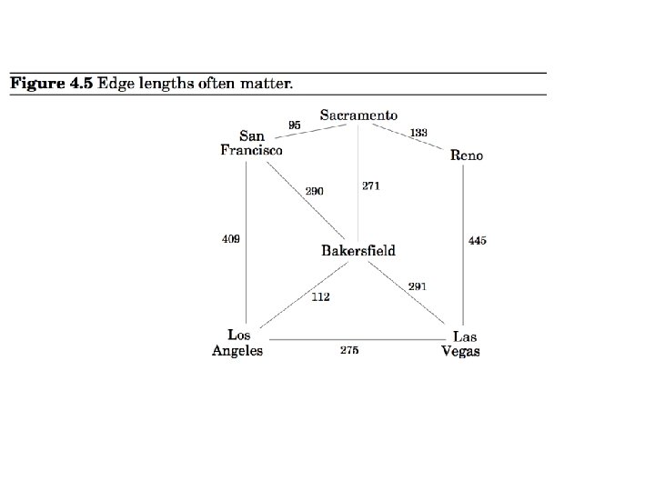
Edges have (positive) lengths • Breadth-first search treats all edges as having the same length. • In reality the edges have lengths, and we are interested in computing shortest paths. • Our graph is a weighted graph G = (V, E) where each edge e = (u, v) of E has length le or we will sometime also write l(u, v) or luv.

Dijkstra’s algorithm • An adaptation of breadth-first search. • Given a weighted graph G, we construct an unweighted graph G’ = (V’, E’) where – For any edge e = (u, v), replace it by le edges of length 1, by adding le -1 dummy nodes between u and v.

A problem with the adaptation • Running time is also dependent on the size of length parameter.

An intuitive description of Dijkstra’s algorithm • I have used the ideas described at: http: //www. quora. com/What-is-the-simplest-intuitive-proof-of-Dijkstra’s-shortest-pathalgorithm

An intuitive description of Dijkstra’s algorithm • We are given a weighted graph G = (V, E), and interested in computing the shortest paths from s (source node). • We drop a huge colony of ants on to the source node s time 0. • They move from there and follow all possible paths through the graph at a rate of one unit per second. • The first one to reach the node v will do so at time dist(s, v). • dist(s, v) is the shortest distance from s to v.

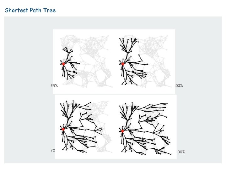
Expanding wavefront of ants

Expanding wavefront of ants

Expanding wavefront of ants

Expanding wavefront of ants

Expanding wavefront of ants

Expanding wavefront of ants

Information to maintain • Two information items we need to maintain: – A schedule to keep track of future arrival of the first ant en route to each node (shown in red in the animation). Initially, the ants are only scheduled to arrive at u at time 0. – A visited array to mark the nodes that ants have already reached (shown as greenish in the animation).

Data structure updates when an ant reach node i at time t. • We will mark node i as visited. • We will remove i from the schedule. • For each edge from i to an unvisited node j, the ants will move down that edge. • Ants are also moving back toward any visited nodes, but we don’t care about these ants since they will never find any new nodes. • We note that ants will arrive at j, from i, at time t + w where w is the length of the edge. – If j is already in the schedule, set dist(j) = min {dist(j), t + w}. – if j is not in the schedule, add j to the schedule with tentative arrival time as t + w, i. e. set dist(j) = t + w.

• We repeat this process with the earliest arrival time of the vertex from the schedule.

// Tins : time per operation //Tex : time per operation // Tdec : time per operation

Three operations on the schedule 1. Remove the entry with earliest time (this happens once for each node). 2. Add a new entry (this happens once for each entry) 3. Decrease the time associated with an existing entry (this happens at most once for each edge)

Using Array Implementations • O(|V|(Tins + Tex) + |E| Tdec) • Implement priority queue with an unsorted array: – – Tins = O(1), Tex = O(|V|), Tdec = O(1) total time is O(|V|2) 46

Running Time using Binary Heaps • O(|V|(Tins + Tex) + E Tdec) • If priority queue is implemented with a binary heap, then – Tins = Tex = Tdec = O(log |V|) – total time is O(|E| log |V|) 47

Running Time using Fibonacci Heaps • O(|V|(Tins + Tex) + E Tdec) • If priority queue is implemented with a Fibonacci heap, then – Tex = O(log |V|) – Tins = Tdec = O(1) – total time is O(|V| log |V| + |E|) 48

Dijkstra's Algorithm Example a 2 iteration 0 b 12 8 10 6 c 3 4 9 2 d e 4 a is source node Q d[c] d[d] d[e] 2 abcde cde d[a] 0 d[b] 1 ∞ ∞ 3 4 5 de d Ø 0 0 0 2 2 2 12 10 10 ∞ ∞ ∞ 16 13 13 11 11 49

Example Will be completed in the class.

Performance Summary • Choice of priority queue implementation directly affects performance. • 2, 000 vertices, 1 million edges: heap 2 -3 times slower than array • 100, 000 vertices, 1 million edges: heap gives 500 x speedup • 1 million vertices, 2 million edges: heap gives 10, 000 x speedup.

Performance Summary • Choice of priority queue implementation directly affects performance. • 2, 000 vertices, 1 million edges: heap 2 -3 times slower than array • 100, 000 vertices, 1 million edges: heap gives 500 x speedup • 1 million vertices, 2 million edges: heap gives 10, 000 x speedup. • array implementation is better for dense graph • heap is better for sparse graph

Shortest paths in the presence of negative cycles • We have implicitly assumed that the shortest path from the starting point s to any node v must pass exclusively through nodes that are close to v. Source A 2 8 5 C B Destination D 7 • Dijkstra’s algorithm returns the path <A, C, D> as the shortest path from source node to destination node.

Shortest paths in the presence of negative cycles • This property is no longer holds when edge length is allowed to be negative. Source A 2 8 5 C B Destination D -7 • Dijkstra’s algorithm still returns the path <A, C, D> as the shortest path from source node to destination node. However, this is incorrect. • Negative edge weights present problems for Dijkstra’s algorithm.

Shortest paths in the presence of negative cycles • A bigger problem is negative cycles like the one below, since this means that there doesn’t exists a true shortest paths. Source A -10 3 15 C B Destination D 5 • We can make the shortest paths as small as possible.

Just add a big number to each edge • Adding a large number M to each edge doesn’t work.

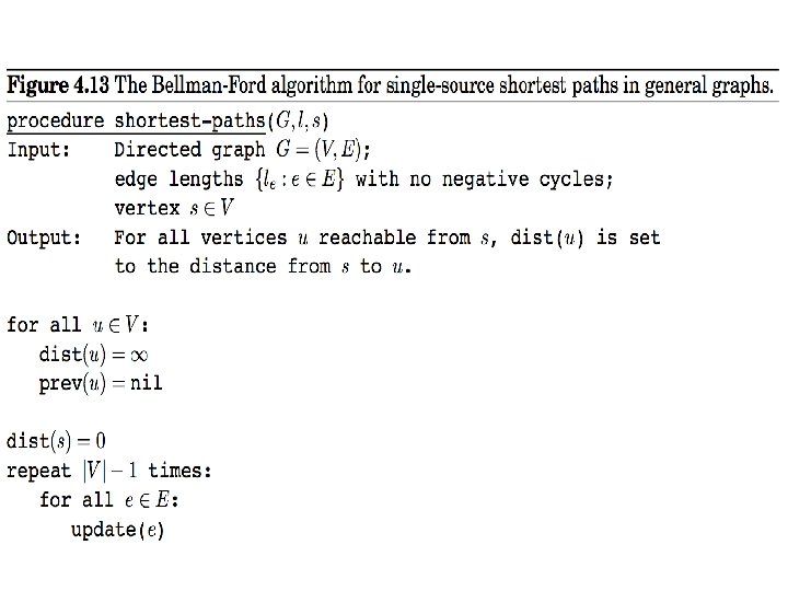
Bellman-Ford Algorithm • Handles graphs with negative edge weights. • It will return the same output as Dijkstra’s for any graphs with positive weights, but run slower.

Edge update v u Update (relaxation) sets dist(v) to the length of a shorter path from s to v.

Edge update • dist(v) is the length of some path from source vertex s to v. • Relaxation (update) along edge e from v to w. – dist(v) is the length of some path from s to v – dist(w) is the length of some path to w –

Bellman-Ford Example 2 B 4 D 4 A 3 -5 1 3 2 C E 5 A B C D E 0 ∞ ∞

Bellman-Ford Example 2 B 4 D 4 A 3 -5 1 3 2 C E 5 A B C D E 0 4 2 ∞ ∞

Bellman-Ford Example 2 B 4 D 4 A 3 -5 1 3 2 C E 5 A B C D E 0 3 2 6 6

Bellman-Ford Example 2 B 4 D 4 A 3 -5 1 3 2 C E 5 A B C D E 0 3 2 1 6

Bellman-Ford Example B 4 A A B C D E 0 ∞ ∞ 0 4 2 ∞ ∞ 0 3 2 6 6 0 3 2 1 6 D 4 3 2 2 -5 1 3 C 5 Each row is one of V-1 iterations Each vertex is updating using values from the previous iteration E

Bellman-Ford algorithm • Running time is O(|E||V|). • Invariant: At end of phase i, dist(v) ≤ length of any path from s to v using at most i edges. • Theorem: If there are no negative cycles, upon termination, dist(v) is the length of the shortest path from s to v.

Bellman-Ford algorithm • Running time is O(|E||V|). • Invariant: At end of phase i, dist(v) ≤ length of any path from s to v using at most I edges. • Theorem: If there are no negative cycles, upon termination, dist(v) is the length of the shortest path from s to v. • Observation: If dist(v) doesn’t change during phase i, there is no need to relax any edge leaving v in phase i+1.

Negative cycles • It can be tested if a given graph has a negative cycle. • Check if Bellman-Ford algorithm updates dist(v) for any v in phase |V|. If it does, the graph has a negative cycle. (why?

Shortest paths in dags • • There is no cycle. Edge weights could be negative. We still cannot use Dijkstra’s algorithm. We can use Bellman-Ford algorithm. – Running time is O(|E||V|) – For dense graphs this is O(|V|3). • We can reduce the complexity to O(|V| + |E|).

Shortest paths in dags • Use the topological order of the vertices of the dags. (Can be done in linear time) – dist(s) = 0 – Determine the topological order of the vertices. (Also known as Linearize G) – for each vertex u of V, in linearized order for all edges (u, v), radiating from u: update(u, v)

Problems from the text • Practice problems (Chapter 4) – 1, 2, 4, 6, 7, 8, 9*, 10, 12, 13, 17, 19, 20