Graphs Chapter 3 Acknowledgement I have used some

Graphs (Chapter 3)

Acknowledgement • I have used some slides from: http: //web. stanford. edu/class/archive/cs/cs 161. 1138/

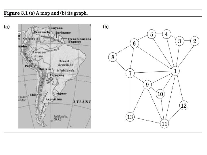
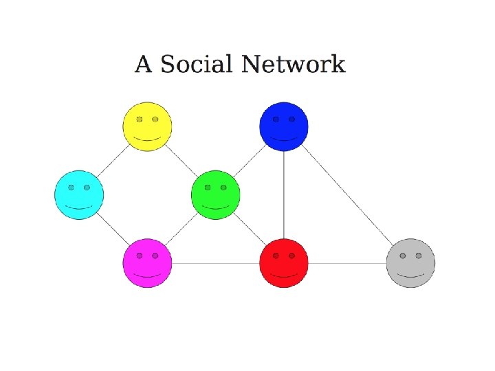
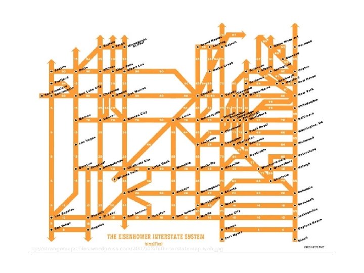
Why Graphs? • Graphs are commonly used to represent varieties of problems.

Some examples • Connected graph • Complete graph

Some examples • Disconnected graph

Some examples • Edge-weighted graph

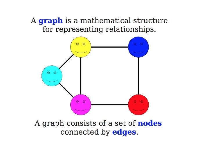
Graph Terminology • A graph is an ordered pair G=(V, E) where – V is the set of vertices (nodes) of the graph – E is the set of edges of the graph • E can be a set of ordered or unordered pairs of vertices: e= {u, v} (undirected}; e=(u, v) (directed). – If E consists of unordered pairs, G is undirected. – If E consists of undirected pairs, G is directed.

Graph Terminology • When analyzing algorithms on a graph, there are usually two parameters we care about: – The number of nodes n. (n = |V|) – The number of edges m, (m = |E|) • Note that m = O(n 2). • A graph is dense if m = Θ(n 2). A graph is called sparse if it is not dense.

Graph Terminilogy • In an undirected graph, the degree of a node (denoted deg(v)) is the number of edges incident to v. • In a directed graph, the indegree of a node (denoted deg-(v)) is the number of edges entering v and the outdegree of a node v (denoted deg+(v)) is the number of edges leaving v.

Some examples • Edge-weighted graph

How is a graph represented? • Adjacency matrix: If there are n = |V| vertices v 1 , v 2 , …, vn , this is an n x n array whose (i, j)th entry is • For undirected graphs, the matrix is symmetric. • For directed graphs the matrix is not symmetric.

Storage space: O(n 2)

Adjacency matrix benefit • The biggest convenience is that the presence of a particular edge can be checked in constant time. • Any algorithm that uses adjacency matrix structure to store a graph has Ω(n 2) lower bound. This is true even if |E| is O(n).

Adjacency list representation • It consists of |V| linked lists, one per vertex. • The linked list for a vertex u holds the names of the vertices to which u has an edge of the type {u, v} or (u, v) of E. • Each edge appears in exactly one of the linked lists if the graph is directed, or two of the lists if the graph is undirected.

Storage space: O(n+m)

Adjacency lists benefits • The storage space requirement is O(n + m), which is optimal in the sense that no other representation taking less than this amount is possible. • Checking of for an edge is no longer a constant time operation. • Iterating through all the neighbors of a vertex is now easy. • An algorithm on a graph runs in linear time if the running time of the algorithm is O(n + m).

Relative advantages of adjacency lists and matrices (From the book: The Algorithm Design Manual by Skienna)

Depth-first search (DFS) in undirected graph • DFS is a versatile linear time procedure to traverse (explore) a graph. • The undirected graph G=(V, E) is represented by an adjacency list. • DFS traverses a graph G = (V, E) in a systematic manner revealing a wealth of information about a graph.

explore(G, v) • Visits the vertices of G, reachable from v. • Input: undirected graph G = (V, E); v V. • Output: visited(u) is set to true for all nodes reachable from v. • The graph is represented an adjacency list structure. • The algorithm is recursive.

explore(G, v) • The algorithm given in the text follows.

An example

explore(G, v) • The algorithm given in the text The previsit(v) and postvisit(v) procedures are optional meant for performing other operations on the vertex v.

explore(G, v) A neat implementation

explore(G, v) A neat implementation

An example

An example parent[A] = nil parent[B] = A parent[E] = A parent[I] = E parent[j] = I

An example parent[A] = nil parent[B] = A parent[E] = A parent[I] = E parent[j] = I • The solid edges are actually those that are traversed, each of which is effected by a call to explore and led to the discovery of a new vertex. These edges form a tree. The edges are call DFS tree edges. • Tree edges are { (parent[u], u)| u, parent[u] is not nill}

dfs(G) • The explore procedure visits only the portion of the graph reachable from its starting point. • To examine the rest of the graph, we need to restart the procedure elsewhere, at some vertex that has not yet been visited.

Procedure dfs(G)

An example

Analysis of dfs(G) • Thanks to the ``visited” array, each vertex is explore’d exactly once. • During the exploration of a vertex, there are the following steps: – Some fixed amount of work – marking the spot as visited, assigning a value to entry, exit array (included in previsit /postvisit section; in the text they are called pre and post times) (O(1) total time per vertex) – A loop in which adjacent edges are scanned, to see if they lead to somewhere new. • Each edge connecting x and y is visited twice: once during explore(G, x) and once during explore(G, y). – The overall time for step 2 over the entire course of dfs(G) is O(|E|). • The worst case running time is O(|V|+|E|). • DFS algorithm is optimal.

Interesting observation of time intervals • The time intervals have interesting and useful properties with respect to a depth-first search. • Who is an ancestor in the DFS tree? – Suppose x is an ancestor of y in DFS tree. This implies that we must visit x before visiting y, and we must exit y before we exit x. Therefore, the time interval [entry[x], exit[x]] contains the time interval [entry[y], exit[y]].

An example

Interesting observation of time intervals • How many descendants? – The difference between the exit (post in the text) and the entry (pre in the text) times for v tells us how many descendants v has in the DFS tree. The clock gets incremented on each vertex entry and vertex exit, so half the time difference denotes the # of descendants of v.

An example

Connectivity in undirected graphs • An undirected graph is connected if there is a path between any pair of vertices. • A connected component of G is a subset C of V with the following properties: – C is nonempty. – For any u, v C: u and v are connected. – For any u C, v V – C: u and v are not connected.

Connectivity in undirected graphs • The following modifications to dfs(G) compute the number of connected components of G.

Depth-first search in directed graphs • For directed graphs, algorithm explore(G, v), designed for undirected graphs earlier, can be used in verbatim.

• • Vertices are picked in lexicographic order. A is the root of the search tree; everything else is its descendants. E has descendants F, H, G, and conversely, is an ancestor of these three nodes. C is the parent of D

Types of edges • Tree edges: Edges lead from a node to its The resulting tree could be disconnected (forest). • Forward edges: Edges lead from a node to a nonchild descendant in DFS tree. • Back edges: Edges lead to an ancestor in the DFS tree • Cross edges: Edges lead to neither descendant nor ancestor.

Types of edges • Tree edges: Edges lead from a node to its The resulting tree could be disconnected (forest). • Forward edges: Edges lead from a node to a nonchild descendant in DFS tree. • Back edges: Edges lead to an ancestor in the DFS tree • Cross edges: Edges lead to neither descendant nor ancestor. • Let u and v be two nodes. Ancestor or descendant relationships can be determined directly from entry (pre) and exit (post) numbers. • Let [u …. ]u denote the time interval for node u. • If the intervals of u and v look like [u … [v … ]u, u is the ancestor of v or v is the descendant of u.

Summary of the various possibilities for an edge (u, v)

Directed acyclic graphs (DAGs) • A graph without a cycle is called acyclic. • G is a DAG if and only if its depth-first search reveals no back edge. This can therefore be tested in optimal O(|V| + |E|) time. In a DAG, every edge leads to a vertex with lower exit (post) number. • DAGs are good for modeling hierarchies and temporal dependencies: course prerequisites, task dependencies etc.

Strongly Connected Components • Directed Conectivity – In a directed graph, we say v is reachable from u if and only if there is a path from u to v. – In an undirected path, if there is a path from u to v, there is also a path from v to u. – In a directed graph, it is possible for v to be reachable from u, but u is not reachable from v. – Two nodes u and v of a directed graph are connected (or strongly connected) if there is a path from u to v and a path from v to u.

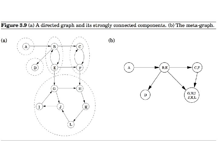
Strongly Connected Components • Let G = (V, E) be a directed graph. • A strongly connected component (or SCC) of G is a subset C of V with the following properties: – C is not empty. – For any u, v C: u and v are strongly connected. – For any u C, v V – C: u and v are not strongly connected.

A directed graph

A directed graph and its strongly connected components

Properties of SCCs • The following properties of SCCs are true. (why? ) – Two SCCs C 1 and C 2 are either equal or disjoint – Every node belongs to exactly one SCC – The SCCs of a graph form a partition of the nodes of the graph.

Condensation (meta) graphs • The condensation of a directed graph G is the directed graph GSCC whose nodes are the SCCs of G and whose edges are defined as follows: (C 1, C 2) is an edge in GSCC iff u C 1, v C 2; (u, v) is an edge in G. • In other words, if there is an edge in G from any node in C 1 to any node in C 2, there is an edge in GSCC from C 1 to C 2.

An important property • The condensation (meta) graph GSCC of any directed graph G is a dag. • Every dag has at least one source node and at least one sink node.

An efficient algorithm to compute the SCCs of a directed graph. • The objective of the algorithm is to identify one of the source nodes in the condensation graph. Once it is identified, it will be removed from G. The process is repeated for the reduced graph. • The objective is to use the depth-first search algorithm which we know runs very fast.

Identify a source strongly connected component • Perform DFS(G) • Find the node with the largest exit (post) time stamp.

Identify a source strongly connected component z lies in a strongly connected component which is a source node in the condensation graph GSCC. • Perform DFS(G) • Find the node z with the largest exit (post) time stamp.

Determine the SCC that contains z z z GSCC • • (GSCC) R Perform DFS on GR from node z where GR is obtained from G = (V, E) by reversing the direction of each edge of G. The search ends after finding the component containing z. The time spent to find this component is proportional to the size of the component. Remove all the nodes from G, reachable from z. Let G’ be the reduced graph.

Repeat the process after removing a component (G’)SCC • • • ((G’)SCC)R Select the next vertex z of G’ with the largest exit time stamp. z now lies in the component which is a source node of (G’)SCC. In the figure it is either B or E. We find all the vertices reachable from z’. These vertices form a strongly connected component.

Algorithm to computing strongly connected components • G is the given directed graph. – – Run DFS on G. Record the exit (post) time stamp of each node. Compute GR Run DFS on GR always starting from the node with the largest exit time stamp. • Since GR can be computed in linear time, the above algorithm runs in linear O(|V| + |E|) time.

Finding Cycles • In an undirected graph, the absence of nontree edges imply nonexistence of cycles. (why? ) • This can be tested by the DFS of the graph.

Topological Sorting • Topological sorting is the most important operation on DAGs. • It orders the vertices on a line such that all directed edges go from left to right. • Such an ordering cannot exist if the graph contains a directed cycle. • The ordering gives us a sequence of processes which can be executed honoring the precedence relation.

Topological Sorting • Topological sorting can be performed efficiently using DFS. • During the DFS when a vertex receives an exit time stamp, append the vertex in the front of linear order linked list. • For exercise 3. 3 of the text, suppose the search starts from A. • The linear order (in reverse order) is : G, H, F, D, E, A, B.

Problems: • Most of the exercise problems in Chapter 3 in the text are interesting and should be solved. The following problems are designated as practice problems. • Chapter 3: 2, 3, 4, 5, 7*, 10, 11*, 12, 14, 16, 18, 21, 22*, 24, 26, 29