Semiclassical Sampling and Linear Inverse Problems Sampling meets

Semiclassical Sampling and Linear Inverse Problems Sampling meets Microlocal Analysis Plamen Stefanov

We heard about sampling for the Radon transform this week in the talks of: • Carl Crawford (sampling; aliasing; our detectors are not points - they have shape) • Alexander Katsevich • Simon Arridge (on the last slide) Aside from this meeting: • Bracewell, 1956 • Rattey & Lindgren, 1981 • Natterer, 1986, 1993 • … and last but not the least…

Use “iradon” in MATLAB to invert the Radon Transform. original Looks good! reconstruction

Increase the frequency. original An artifact! reconstruction

Increase the frequency even more. original The artifact moved closer! reconstruction

… and even more. . . original Two artifacts! reconstruction

reconstruction original
")
and (unitarity)

Graph of sinc
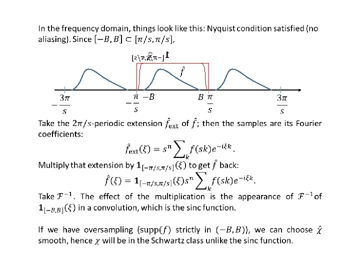

Aliasing: If the Nyquist condition is not satisfied:

Oversampled on 81 x 81 grid Undersampled on 41 x 41 grid The original consist of two patterns: one higher frequency than the other. First, we sample and reconstruct properly. Next, we undersample the higher frequency pattern but still sample properly the lower frequency one. The reconstruction changes the direction and the frequency of the undersampled pattern. The Fourier transforms demonstrate the shifting (folding) of the frequencies.

This brings us to the first problem we need to study: • Uniform sampling on rectangular or non-rectangular lattices? • Non-uniform sampling? • How many sampling points are enough?
 Semi-classical sampling")
(v) Semi-classical sampling
 Semi-classical sampling The sampling lattice The Fourier domain")
(v) Semi-classical sampling The sampling lattice The Fourier domain
 Semi-classical sampling The sampling lattice The lattice could be rectangular The Fourier domain")
(v) Semi-classical sampling The sampling lattice The lattice could be rectangular The Fourier domain
 Semi-classical sampling The sampling lattice The Fourier domain")
(v) Semi-classical sampling The sampling lattice The Fourier domain
 Semi-classical sampling")
(v) Semi-classical sampling
 Semi-classical sampling We have the following microlocal analog of this result.")
(v) Semi-classical sampling We have the following microlocal analog of this result.
 Sampling FIOs")
(i) Sampling FIOs

Example 1: The Radon transform in “parallel geometry”
 Sampling")
Radon transform: (i) Sampling
 Sampling")
Radon transform: (i) Sampling
 Sampling")
Radon transform: (i) Sampling
 Resolution Circular lines well resolved. Radial not. best resolution uniform blur")
Radon transform: (ii) Resolution Circular lines well resolved. Radial not. best resolution uniform blur plus non-local artifacts original
 Aliasing")
(iii) Aliasing
 Aliasing")
(iii) Aliasing
 Aliasing")
Radon transform: (iii) Aliasing
 Aliasing reconstruction original")
Radon transform: (iii) Aliasing reconstruction original
 Aliasing reconstruction original The higher frequency pattern disappears! It actually shifts")
Radon transform: (iii) Aliasing reconstruction original The higher frequency pattern disappears! It actually shifts out of the computational domain.
 Averaged measurements")
(iv) Averaged measurements
 Averaged data original")
Radon transform: (iv) Averaged data original

Example 2: The Radon transform in “fan-beam geometry”
 Sampling")
Fan-beam geometry: (i) Sampling
 Sampling")
Fan-beam geometry: (i) Sampling
 Resolution The diagram is rotationally symmetric.")
Fan-beam geometry: (ii) Resolution The diagram is rotationally symmetric.
 Aliasing")
Fan-beam geometry: (iii) Aliasing
 averaged data The levels sets are as in the resolution analysis.")
Fan-beam geometry: (iv) averaged data The levels sets are as in the resolution analysis. Unlike in the parallel geometry case, those terms are different! They blur differently and then the results are added.
 averaged data (a) original (b) Radial blur. Corresponds to the red")
Fan-beam geometry: (iv) averaged data (a) original (b) Radial blur. Corresponds to the red bars. (c) Sum of two blurs. Corresponds to the circles. (d) Source restricted to the right semi-circle. We get better resolution near the source (direction dependent). Corresponds to one of the circles only. The resolution diagram
 averaged data A magnified crop")
Fan-beam geometry: (iv) averaged data A magnified crop

Fan-beam geometry: anti-aliasing original A lot of aliasing artifacts spreading everywhere The anti-aliasing removes most of the artifacts but softens the image a bit more.

Thermo-acoustic Tomography

Thermo-acoustic Tomography
. Much higher frequencies, needs finer")
Thermo-acoustic Tomography Fast region inside, no caustics (before reflections). Much higher frequencies, needs finer sampling.
- Slides: 46