SAR Algorithms Recap What is SAR processing SAR

SAR Algorithms

Recap: What is SAR processing? • SAR processing algorithms model the scene as a set of discrete point targets that do not interact with each other (aka Born approximation) • No multibounce • The electric field at the target comes only from the incident wave and not from surrounding scatterers • The target model is linear because the scattered response from point target P 1 and point target P 2 is modelled as the response from point target P 1 by itself + response from point target P 2 by itself • We can apply the principle of superposition!!! • SAR processing is the application of a matched filter for each pixel in the image where the matched filter coefficients are the response from a single isolated point target • We will assume noise is whitened (decorrelated) • Equivalently, we can say: • SAR processing is a correlation filter between a single isolated point target response and the raw data • SAR processing is an inner product between our model of a single isolated point target and the raw data

Recap: What is SAR processing? • SAR processing algorithms model the scene as a set of discrete point targets that do not interact with each other (aka Born approximation) • No multibounce • The target’s electric field is only from the incident wave and not from surrounding scatterers • The target model is linear because the scattered response from point target P 1 and point target P 2 is modelled as the response from point target P 1 by itself + response from point target P 2 by itself • We can apply the principle of superposition!!! • SAR processing is the application of a matched filter for each pixel in the image where the matched filter coefficients are the single isolated point target response • We will assume noise is whitened (decorrelated) • Equivalently, we can say: • SAR processing is a correlation filter between a single isolated point target response and the raw data • SAR processing is an inner product between our model of a single isolated point target and the raw data

Recap: What is SAR processing? • SAR processing algorithms model the scene as a set of discrete point targets that do not interact with each other (aka Born approximation) • No multibounce • The target’s electric field is only from the incident wave and not from surrounding scatterers • The target model is linear because the scattered response from point target P 1 and point target P 2 is modelled as the response from point target P 1 by itself + response from point target P 2 by itself • We can apply the principle of superposition!!! • SAR processing is the application of a matched filter for each pixel in the image where the matched filter coefficients are the single isolated point target response • We will assume noise is whitened (decorrelated) • Equivalently, we can say: • SAR processing is a correlation filter between a single isolated point target response and the raw data • SAR processing is an inner product between our model of a single isolated point target and the raw data

Recap: What is SAR processing? • So… SAR processing is a matched filter and the filter is linear • If the filter was also space invariant we could apply it in the frequency domain • But: the filter is not space invariant. The point target’s shape changes depending on the range to the radar.

Why do we care that it is not space invariant? • Recall linear time invariant (LTIV) systems have complex exponentials as their Eigenfunctions. A change of basis of the input and output to complex exponentials means that a simple component-wise multiply is all that is needed to apply the filter. A change of basis to complex exponentials can be efficiently implemented using a Fast Fourier Transform (FFT) assuming data are uniformly sampled. • Without Fourier method, O(N 2 M 2) operations are required instead of O(N*log 2(N) M*log 2(M)) where N and M are the dimensions of the image and are usually on the order of thousands of pixels each. The direct application of “slow” convolution could be more than 100 x slower than “fast” or Fourier based convolution. • Good news: we can exploit the structure of the signal to transform (usually through interpolation) the data into a domain where the signal is space invariant! To do this, we require properly sampled raw data and image pixels.

Principle of Stationary Phase (PSOP) •

Remember: must include your original phase function being integrated AND the Fourier term: 1. Write out envelope and phase function 2. Determine derivative of phase function. 3. Solve for the stationary point, ts, in terms of f. This is the first messy part… 4. Determine second derivative of phase function. IGNORED IN OUR DERIVATIONS! 5. Plug t(f) into (4) wherever the stationary point occurs. 6. Simplify! This is the second messy part… Process is the same for inverse Fourier transform except replace eqns above with:

Good online SAR Resource • https: //saredu. dlr. de/unit

Satellite and Low Squint Airborne SAR Algorithms • Lower squint (often <4 -5 deg) • Narrow azimuth bandwidth (usually 0. 5 deg to 10 deg azimuth beamwidth) • Range Doppler Algorithm • Used by the Canadian Space Agency to process RADARSAT-1 and RADARSAT-2 satellite SAR data • Chirp Scaling Algorithm • Used by the European Space Agency and the German Aerospace Center (DLR) to process Terra. SAR-X satellite SAR data • These two algorithms (RDA and CSA) are very similar with the primary difference being how range cell migration correction is done. • RDA works with any waveform, CSA requires the use of a chirp waveform

Satellite and Low Squint Airborne SAR Algorithms • The SAR filter is azimuth-space-invariant but it is range-variant • The primary structure exploited by these two algorithms is that the 2 D energy from the point target lies along a 1 -D contour. This energy will be interpolated or scaled/shifted to lie on a 1 -D line that does not cross range bins. By converting the range varying dimension to lie on a single range bin, convolution will no longer be required in the range dimension.

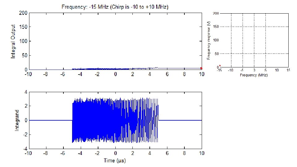
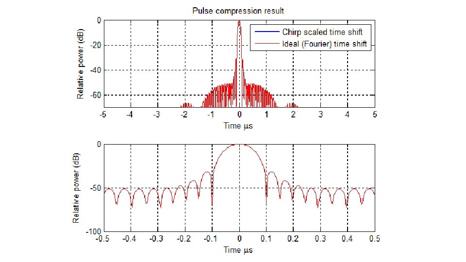
Range Doppler Algorithm (RDA) STEP 1 • Pulse compression is a LTIV filter. It is straight forward to implement in the Fourier domain. • Range FFT on raw data to transform to range-frequency / azimuth-space domain • Apply range-domain matched filter for pulse compression • Do not take the IFFT in the range dimension when finished.

Range Doppler Algorithm (RDA) STEP 2 • Azimuth FFT • Transform to range-frequency / Doppler domain Raw Data (single target) 2 D Fourier Domain (3 targets)

Range Doppler Algorithm (RDA): STEP 3 • Blurring occurs during the Doppler Fourier transform so that the point target “contour” is broadened. This affect is worse for large squint angles. • This blurring can be approximated by a frequency chirp in the range domain… so to correct we need to do pulse compression again. • This process is called Secondary Range Compression • For an approximate solution, this second range compression can be applied during the regular pulse compression… this is suboptimal because the Fourier transform to the Doppler domain blurs the correction so it is better to apply in the range-Doppler domain.

Range Doppler Algorithm (RDA): STEP 3 Range Space Domain (i. e. Raw Data) Range Doppler Domain (note the blurring)

Range Doppler Algorithm (RDA): STEP 3 •

Range Doppler Algorithm (RDA): STEP 3 Range Doppler Domain (After Secondary Range Compression) Range Doppler Domain (note the blurring)

Range Doppler Algorithm (RDA): STEP 4 • Range IFFT • Transform to range / Doppler domain

Range Doppler Algorithm (RDA): STEP 5 • Range Cell Migration Correction (RCMC) in Doppler domain • SAR processing is a 2 -D filter, but the energy is focused along a single hyperbolic contour. • Contour is range dependent • The idea is to flatten the contour using a process called RCMC • Example point target response: • RCMC easy to apply for a single point target.

Range Doppler Algorithm (RDA): STEP 5 • Example of two point targets at the same range and next to each other. Envelope is about the same for both but the phases are offset (think of two tones and what you see is the beat frequency… double side band suppressed carrier). • Could apply RCMC for this case as well.

Range Doppler Algorithm (RDA): STEP 5 • Example of two point targets far apart from each other… RCMC not possible because each target needs a different correction.

Range Doppler Algorithm (RDA): STEP 5 • Example of two point targets far apart from each other:

Range Doppler Algorithm (RDA): STEP 5 • RCMC cannot be applied in the range-space domain because RCMC is dependent on the relative along-track position rather than the absolute along-track position. • Hmmm… we know that the range cell migration is a function of incidence angle (i. e. Doppler). • RCMC can be applied in the range-Doppler domain because RCMC depends on the absolute Doppler. • Every target at the same range has the same envelope in the range. Doppler domain!!!

Range Doppler Algorithm (RDA): STEP 5 Single Target Both Targets… envelope has not changed, but interference pattern has.

Range Doppler Algorithm (RDA): STEP 5 •

Range Doppler Algorithm (RDA): STEP 5 • Use the truncated and windowed sinc interpolation method to do the time shift. Example of 3 deg squint:

Range Doppler Algorithm (RDA): STEP 5 • Use the truncated and windowed sinc interpolation method to do the time shift. Example of 10 deg squint:

Range Doppler Algorithm (RDA): STEP 6 • All targets have been interpolated so that they occupy a single range bin in the range-Doppler domain. • Originally the problem was that the range cell migration changed as a function of range This prevented a simple application of Fourier methods since the response was space-variant. • Now it is no longer a 2 -D filter so the space variance does not matter and we only need to apply a 1 -D azimuth filter.

Range Doppler Algorithm (RDA): STEP 6 •

Range Doppler Algorithm (RDA): STEP 7 • Azimuth IFFT • Transform into range / azimuth-space domain

Range Doppler Algorithm (RDA): STEP 7 • Example (side note: range dependent Doppler centroid correction and relative range cell migration correction when there is squint). No squint: Position is perfect 3 deg squint: range is correct, but azimuth is off by one pixel

Range Doppler Algorithm (RDA): STEP 7 10 deg squint (RCMC not perfect) Azimuth correction ends with smeared range bins

Chirp Scaling Algorithm (CSA) • The problem with RDA is that the RCMC interpolation is slow and requires SRC. • Chirp scaling does the same thing as RDA, but does the RCMC with chirp scaling which also makes the blurring from the Doppler Fourier transform smaller. • Greater efficiency + range/azimuth decoupling built into range compression (analogous to range Doppler algorithms secondary range compression)

Chirp Scaling Algorithm (CSA): Step 1 • Azimuth FFT • Transform to range / Doppler domain

Chirp Scaling Algorithm (CSA): Step 2 •

Chirp Scaling Algorithm (CSA): Step 2 •

Chirp Scaling Algorithm (CSA): Step 3 • Range FFT • Transform to range-frequency / Doppler domain

Chirp Scaling Algorithm (CSA): Step 4 •

Chirp Scaling Algorithm (CSA): Step 5 • Range IFFT • Transform to range / Doppler domain

Chirp Scaling Algorithm (CSA): Step 6 •

Chirp Scaling Algorithm (CSA): Step 7 • Azimuth IFFT • Transform to range / azimuth-space domain

Wide Aperture (Airborne and Ground based) Algorithms • f-k migration (AKA -k migration as in omega-wavenumber migration) • Handles strip map mode data collection with very wide apertures • Disadvantage is that time and space variant modifications are not handled well because processing is done in the f-k domain. • Time domain correlation (TDC): not covered • Fast factorized TDC is a good and fast implementation of TDC which keeps most of the desirable properties of TDC • Lars M. H. Ulander et al. , Synthetic-Aperture Radar Processing Using Fast Factorized Back. Projection, Transactions on Aerospace and Electronic Systems, vol. 39, no. 3, July 2003. • Polar Format Algorithm (PFA) : not covered • Armin W. Doerry, Synthetic Aperture Radar Processing with Tiered Subapertures, Sandia Report SAND 94 -1390, 1994. • Very complete description of PFA • Jack L. Walker, Range-Doppler Imaging of Rotating Objects, IEEE Transactions on Aerospace and Electronic Systems, vol. 16, no. 1, Jan 1980. • Original reference.

F-k migration • Exploding reflector model • The linear target model is equivalent to the exploding reflector model • Rather than the radar transmitting a pulse at time zero, each target is replaced by an isotropic source that radiates a pulse starting at time zero and the velocity of propagation is halved.

F-k migration: Step 1 • Two-dimensional FFT • Transform to range-frequency / wavenumber domain • (Wavenumber has a one to one mapping with Doppler domain)

F-k migration: Step 2 • Reference frequency multiply (RFM) • Applies the 2 -D filter for the reference range (i. e. determine the response from a point target at the reference range and then use that as a correlation/matched filter) • This will apply both range and azimuth compression • We know that this will perfectly focus the reference range, but slowly degrade away from that range because the filter needs to be space variant to perfectly focus the targets

F-k migration: Step 2 •

F-k migration: Step 2 • Examples of reference range and away from reference range

F-k migration: Step 3 •

F-k migration: Step 3 •

F-k migration: Step 4 • Two-dimensional IFFT • Transform to range-space domain • Before and after Stolt interpolation for target a long way from the reference range.