Running Time The running time of an algorithm

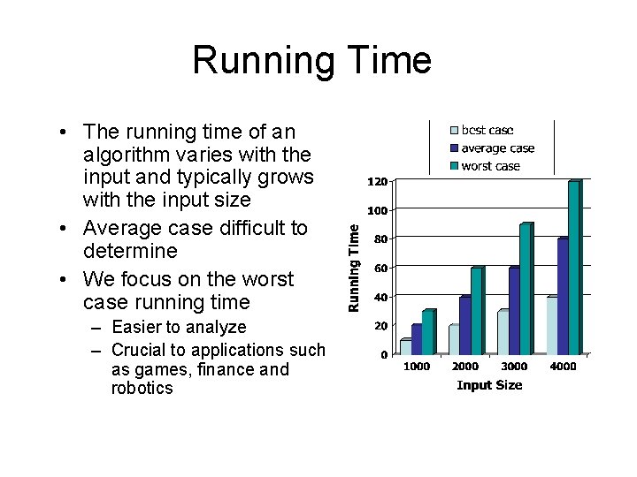
Running Time • The running time of an algorithm varies with the input and typically grows with the input size • Average case difficult to determine • We focus on the worst case running time – Easier to analyze – Crucial to applications such as games, finance and robotics

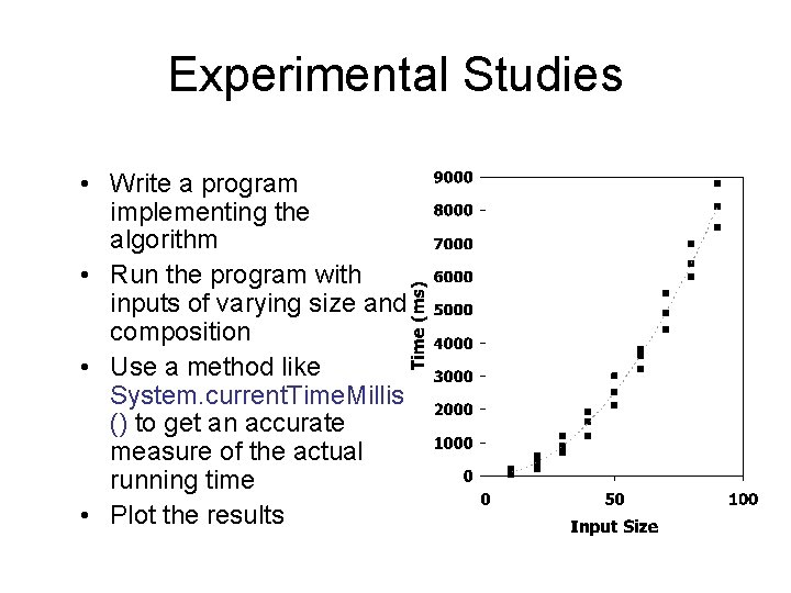
Experimental Studies • Write a program implementing the algorithm • Run the program with inputs of varying size and composition • Use a method like System. current. Time. Millis () to get an accurate measure of the actual running time • Plot the results

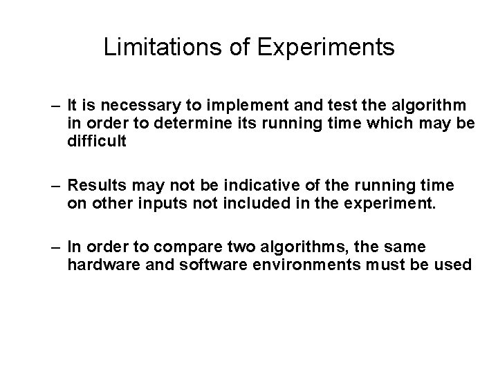
Limitations of Experiments – It is necessary to implement and test the algorithm in order to determine its running time which may be difficult – Results may not be indicative of the running time on other inputs not included in the experiment. – In order to compare two algorithms, the same hardware and software environments must be used

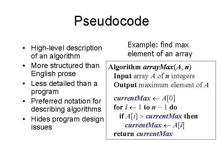
Pseudocode Example: find max • High-level description element of an array of an algorithm • More structured than Algorithm array. Max(A, n) English prose Input array A of n integers • Less detailed than a Output maximum element of A program current. Max A[0] • Preferred notation for i 1 to n 1 do describing algorithms if A[i] current. Max then • Hides program design current. Max A[i] issues return current. Max

Pseudocode Details • Control flow – – – if … then … [else …] while … do … repeat … until … for … do … Indentation replaces braces • Method declaration Algorithm method (arg [, arg…]) Input … Output … • Method call var. method (arg [, arg…]) • Return value return expression • Expressions Assignment (like in Java) Equality testing (like in Java) n 2 Superscripts and other mathematical formatting allowed

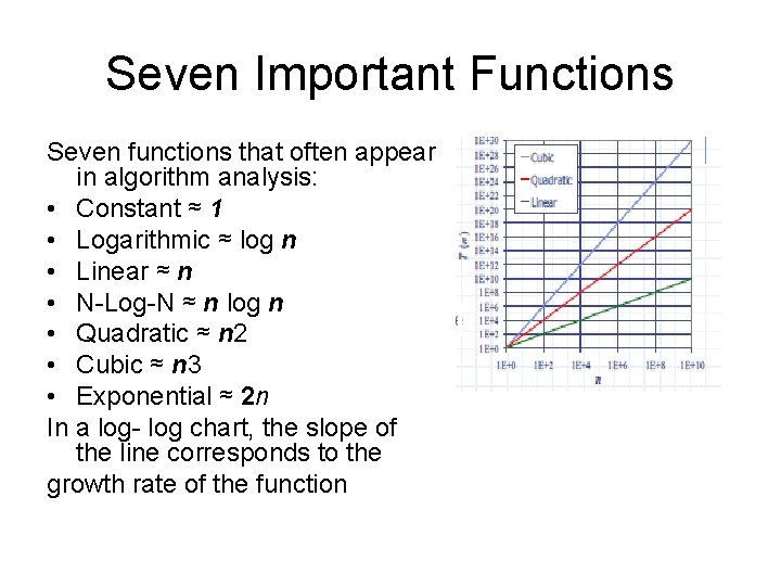
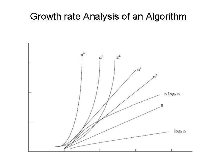
Seven Important Functions Seven functions that often appear in algorithm analysis: • Constant ≈ 1 • Logarithmic ≈ log n • Linear ≈ n • N-Log-N ≈ n log n • Quadratic ≈ n 2 • Cubic ≈ n 3 • Exponential ≈ 2 n In a log- log chart, the slope of the line corresponds to the growth rate of the function

Growth rate Analysis of an Algorithm

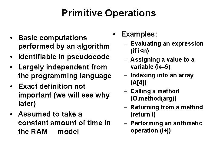
Primitive Operations • Examples: • Basic computations – Evaluating an expression performed by an algorithm (if i<n) • Identifiable in pseudocode – Assigning a value to a variable (i 5) • Largely independent from – Indexing into an array the programming language (A[4]) • Exact definition not – Calling a method important (we will see why (O. method(arg)) later) – Returning from a method • Assumed to take a (return i) constant amount of time in – Performing an arithmetic operation (i+j) the RAM model

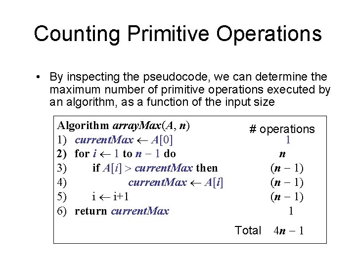
Counting Primitive Operations • By inspecting the pseudocode, we can determine the maximum number of primitive operations executed by an algorithm, as a function of the input size Algorithm array. Max(A, n) 1) current. Max A[0] 2) for i 1 to n 1 do 3) if A[i] current. Max then 4) current. Max A[i] 5) i i+1 6) return current. Max # operations 1 n (n 1) 1 Total 4 n 1

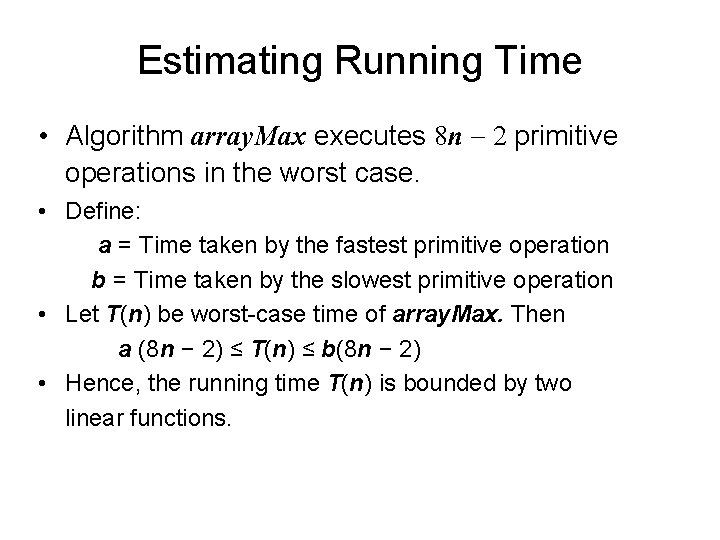
Estimating Running Time • Algorithm array. Max executes 8 n 2 primitive operations in the worst case. • Define: a = Time taken by the fastest primitive operation b = Time taken by the slowest primitive operation • Let T(n) be worst-case time of array. Max. Then a (8 n − 2) ≤ T(n) ≤ b(8 n − 2) • Hence, the running time T(n) is bounded by two linear functions.

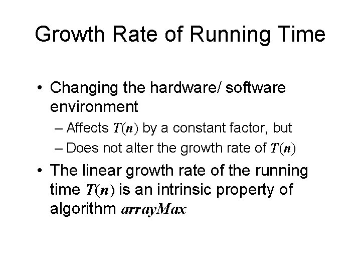
Growth Rate of Running Time • Changing the hardware/ software environment – Affects T(n) by a constant factor, but – Does not alter the growth rate of T(n) • The linear growth rate of the running time T(n) is an intrinsic property of algorithm array. Max

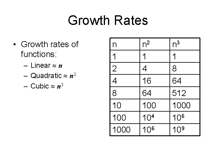
Growth Rates • Growth rates of functions: – Linear n – Quadratic n 2 – Cubic n 3 n 1 2 4 8 10 1000 n 2 1 4 16 64 100 104 106 n 3 1 8 64 512 1000 106 109

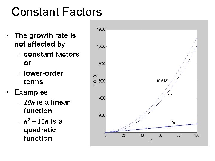
Constant Factors • The growth rate is not affected by – constant factors or – lower-order terms • Examples – 10 n is a linear function – n 2 + 10 n is a quadratic function

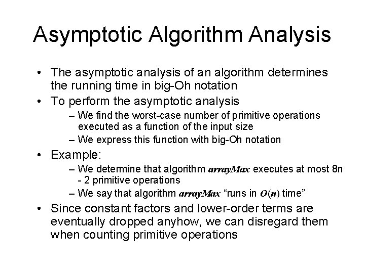
Asymptotic Algorithm Analysis • The asymptotic analysis of an algorithm determines the running time in big-Oh notation • To perform the asymptotic analysis – We find the worst-case number of primitive operations executed as a function of the input size – We express this function with big-Oh notation • Example: – We determine that algorithm array. Max executes at most 8 n - 2 primitive operations – We say that algorithm array. Max “runs in O(n) time” • Since constant factors and lower-order terms are eventually dropped anyhow, we can disregard them when counting primitive operations

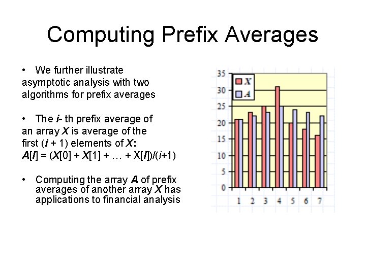
Computing Prefix Averages • We further illustrate asymptotic analysis with two algorithms for prefix averages • The i- th prefix average of an array X is average of the first (i + 1) elements of X: A[i] = (X[0] + X[1] + … + X[i])/(i+1) • Computing the array A of prefix averages of another array X has applications to financial analysis

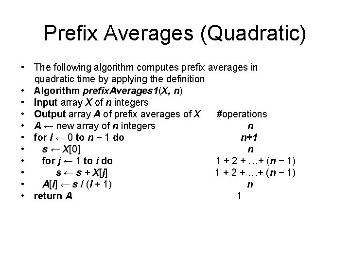
Prefix Averages (Quadratic) • The following algorithm computes prefix averages in quadratic time by applying the definition • Algorithm prefix. Averages 1(X, n) • Input array X of n integers • Output array A of prefix averages of X #operations • A ← new array of n integers n • for i ← 0 to n − 1 do n+1 • s ← X[0] n • for j ← 1 to i do 1 + 2 + …+ (n − 1) • s ← s + X[j] 1 + 2 + …+ (n − 1) • A[i] ← s / (i + 1) n • return A 1

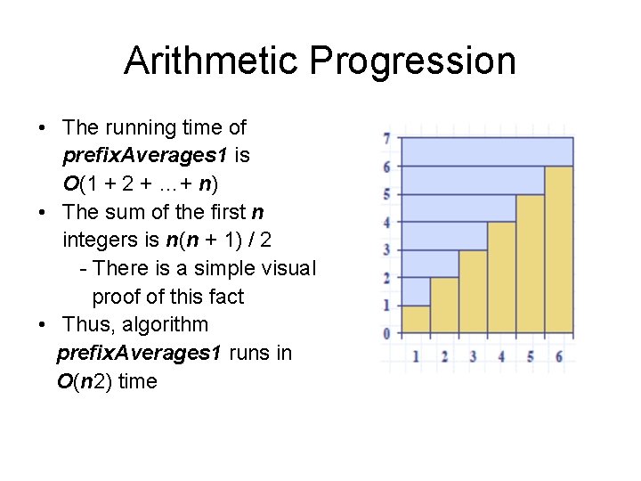
Arithmetic Progression • The running time of prefix. Averages 1 is O(1 + 2 + …+ n) • The sum of the first n integers is n(n + 1) / 2 - There is a simple visual proof of this fact • Thus, algorithm prefix. Averages 1 runs in O(n 2) time

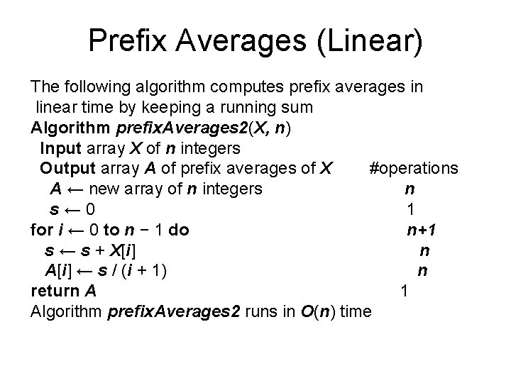
Prefix Averages (Linear) The following algorithm computes prefix averages in linear time by keeping a running sum Algorithm prefix. Averages 2(X, n) Input array X of n integers Output array A of prefix averages of X #operations A ← new array of n integers n s← 0 1 for i ← 0 to n − 1 do n+1 s ← s + X[i] n A[i] ← s / (i + 1) n return A 1 Algorithm prefix. Averages 2 runs in O(n) time

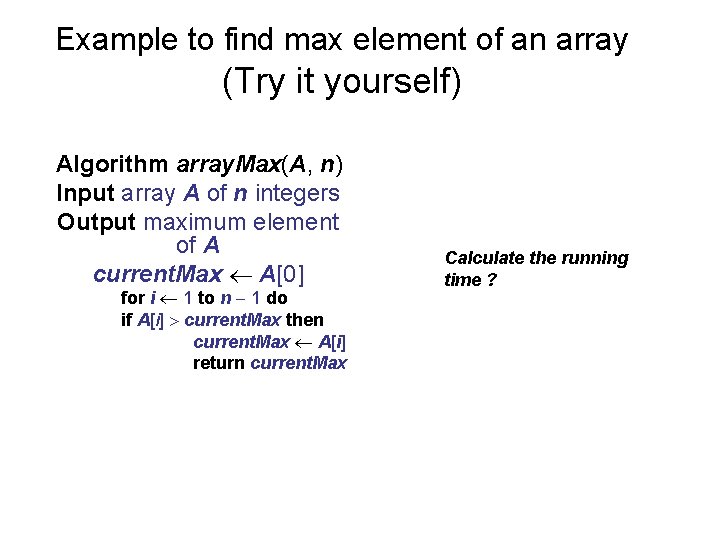
Example to find max element of an array (Try it yourself) Algorithm array. Max(A, n) Input array A of n integers Output maximum element of A current. Max A[0] for i 1 to n 1 do if A[i] current. Max then current. Max A[i] return current. Max Calculate the running time ?