RepeatedMeasures Designs GLM 4 Prof Andy Field Aims

Repeated-Measures Designs (GLM 4) Prof. Andy Field

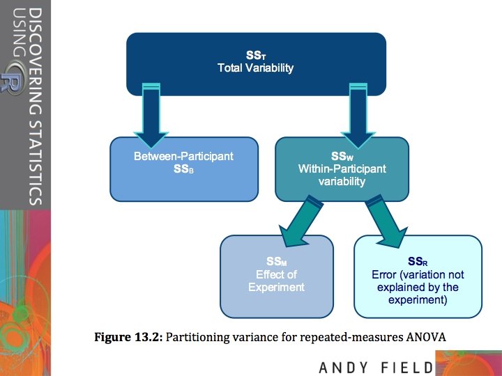
Aims • Rationale of repeated measures ANOVA – One- and two-way – Benefits • Partitioning variance • Statistical problems with repeatedmeasures designs – Sphericity – Overcoming these problems • Interpretation Slide 2

Benefits of Repeated Measures Designs • Sensitivity – Unsystematic variance is reduced. – More sensitive to experimental effects. • Economy – Fewer participants are needed. – But be careful of fatigue. Slide 3

An Example • Are certain bushtucker foods more revolting than others? • Four foods tasted by eight celebrities: – – Stick insect Kangaroo testicle Fish eyeball Witchetty grub • Outcome: – Time to retch (seconds) Slide 4

The Data

Problems with Analysing Repeated-Measures Designs • Same participants in all conditions – Scores across conditions correlate. – Violates assumption of independence (lecture 2). • Assumption of sphericity – Crudely put: the correlation across conditions should be the same. – Adjust degrees of freedom. Slide 7

Exploring the Data Slide 8

Exploring the Data by(long. Bush$Retch, long. Bush$Animal, stat. desc)

The Assumption of Sphericity • Basically means that the correlation between treatment levels is the same. • Actually, it assumes that variances in the differences between conditions is equal. • Measured using Mauchly’s test. – p <. 05, sphericity is violated. – p >. 05, sphericity is met. Slide 10

What is Sphericity? Slide 11 Testicle – Stick Eye – Stick Witchetty – Stick Eye – Testicle Witchetty – Testicle – Eye 1 -1 -7 -2 -6 -1 5 2 -4 -7 -4 -3 0 3 3 -4 -3 2 1 6 5 4 -2 -4 4 -2 6 8 5 -4 -3 0 1 4 3 6 -2 -1 0 1 2 1 7 -8 -3 -8 5 0 -5 8 -6 -4 -11 2 -5 -7 Variance 5. 27 4. 29 25. 70 11. 55 14. 29 26. 55

Estimates of Sphericity • Three measures: – Greenhouse–Geisser estimate – Huynh–Feldt estimate – Lower-bound estimate • Multiply df by these estimates to correct for the effect of sphericity. • G-G is conservative, and H-F liberal. Slide 12

Correcting for Sphericity df = 3, 21 Slide 13

Choosing Contrasts Partvs. Whole<-c(1, -1, 1) Testiclevs. Eye<-c(0, -1, 1, 0) Stickvs. Grub<-c(-1, 0, 0, 1) contrasts(long. Bush$Animal)<-cbind(Partvs. Whole, Testiclevs. Eye, Stickvs. Grub) Slide 14

The Easier (But Slightly Limited) Way: Repeated-Measures ANOVA bush. Model<-ez. ANOVA(data = long. Bush, dv =. (Retch), wid =. (Participant), within =. (Animal), detailed = TRUE, type = 3) • To see the output execute the model name: bush. Model

Output

Post Hoc Tests pairwise. t. test(long. Bush$Retch, long. Bush$Animal, paired = TRUE, p. adjust. method = "bonferroni")

The Slightly More Complicated Way: the Multilevel Approach • We can use lme(): bush. Model<-lme(Retch ~ Animal, random = ~1|Participant/Animal, data = long. Bush, method = "ML") • We have defined the model in exactly the same was as for aov(), we have simply added in a term that lets the model know that the variable Animal is made up of the same participants repeated multiple times across the variable Animal: (random = ~1|Participant/Animal).

The Slightly More Complicated Way: the Multilevel Approach • To test whether Animal had an overall effect, compare the model that we have just created to one in which the predictor is absent: baseline<-lme(Retch ~ 1, random = ~1|Participant/Animal, data = long. Bush, method = "ML") anova(baseline, bush. Model)

Parameter Estimates summary(bush. Model)

Post Hoc Tests • To get post hoc tests for the current data, execute: post. Hocs<-glht(bush. Model, linfct = mcp(Animal = "Tukey")) summary(post. Hocs) confint(post. Hocs)

Post Hoc Tests Output

Robust One-Way Repeated. Measures ANOVA • Needs data to be in wide format. • Get rid of participant variable: bush. Data 2<-bush. Data[, -c(1)]

Robust One-Way Repeated. Measures ANOVA rmanova(bush. Data 2) • or: rmanovab(bush. Data 2, nboot = 2000)

Output

What is Two-Way Repeated. Measures ANOVA? • Two independent variables – Two-way = 2 IVs – Three-way = 3 IVs • The same participants in all conditions – Repeated measures = ‘same participants’ – A. k. a. ‘within-subjects’ Slide 26

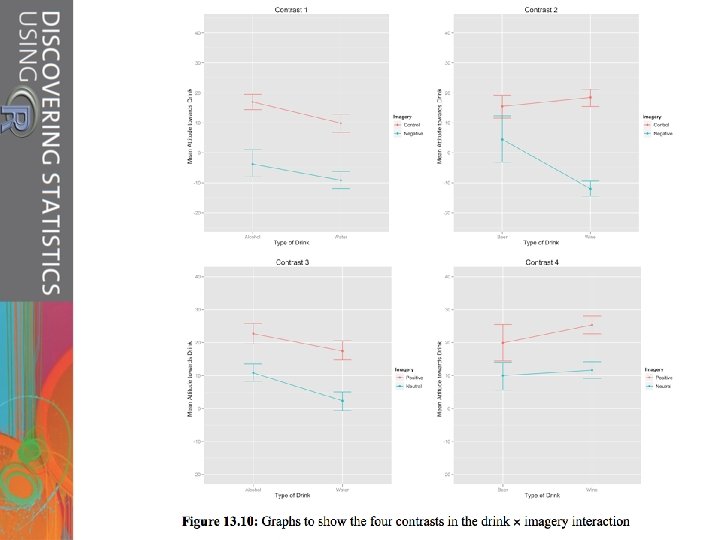
An Example • Field (2009): Effects of advertising on evaluations of different drink types. – IV 1 (Drink): beer, wine, water – IV 2 (Imagery): positive, negative, neutral – Dependent variable (DV): Evaluation of product, from – 100, dislike very much, to +100, like very much Slide 27

SST Variance between all participants SSR SSM Between. Participant Variance Within-Participant Variance explained by the experimental manipulations SSA B Effect of Drink Effect of Imagery Effect of Interaction SSRA SSRB SSRA B Error for Drink Slide 28 SSB Error for Imagery Error for Interaction

Getting Data into the Correct Format • Data needs to be in long format. • Can use melt() function to change data into long format: long. Attitude <-melt(attitude. Data, id = "participant", measured = c( "beerpos", "beerneg", "beerneut", "winepos", "wineneg", "wineneut", "waterpos", "waterneg", "waterneu")) • Rename columns so that we actually know what they represent by executing: names(long. Attitude)<-c("participant", "groups", "attitude") Slide 29

Getting Data into the Correct Format for the Analysis • The variable groups is a mixture of our two predictor variables (imagery and type of drink). • We need to create two variables that dissociate the type of imagery from the type of drink: – long. Attitude$drink<-gl(3, 60, labels = c("Beer", "Wine", "Water")) • We also need a variable that tells us the type of imagery that was used: long. Attitude$imagery<-gl(3, 20, 180, labels = c("Positive", "Negative", "Neutral"))

Getting Data into the Correct Format for the Analysis

Exploring Data Slide 32

Setting Contrasts

Factorial Repeated-Measures ANOVA attitude. Model<-ez. ANOVA(data = long. Attitude, dv =. (attitude), wid =. (participant), within =. (imagery, drink), type = 3, detailed = TRUE) attitude. Model Slide 34

Output

Main Effect of Drink F(2, 38) = 5. 11, p <. 05 Slide 36

Main Effect of Imagery F(2, 38) = 122. 56, p <. 001 Slide 37

The Interaction Effect (drink × imagery) F(4, 76) = 17. 15, p <. 001 Slide 38

Post Hoc Tests for the Interaction Term pairwise. t. test(long. Attitude$attitude, long. Attitude$groups, paired = TRUE, p. adjust. method = "bonferroni")

Factorial Repeated-Measures Designs as a GLM baseline<-lme(attitude ~ 1, random = ~1|participant/drink/imagery, data = long. Attitude, method = "ML") • If we want to see the overall effect of each predictor then we need to add them one at a time: – drink. Model<-update(baseline, . ~. + drink) – imagery. Model<-update(drink. Model, . ~. + imagery) – attitude. Model<-update(imagery. Model, . ~. + drink: imagery)

Factorial Repeated-Measures Designs as a GLM • To compare these models we can list them in the order in which we want them compared in the anova() function: anova(baseline, drink. Model, imagery. Model, attitude. Model)

Parameter Estimates • We can further explore the model by executing: summary(attitude. Model) • Most important, these include the parameters for the contrasts that we set for each variable.

Parameter Estimates