Exploratory Factor Analysis Prof Andy Field Aims Explore

Exploratory Factor Analysis Prof. Andy Field

Aims • Explore factor analysis and principal component analysis (PCA) • What Are factors? • Representing factors – Graphs and Equations • Extracting factors – Methods and Criteria • Interpreting factor structures – Factor Rotation • Reliability – Cronbach’s alpha Slide

When and Why? • To test for clusters of variables or measures. • To see whether different measures are tapping aspects of a common dimension. – E. g. Anal-Retentiveness, Number of friends, and social skills might be aspects of the common dimension of ‘statistical ability’ Slide

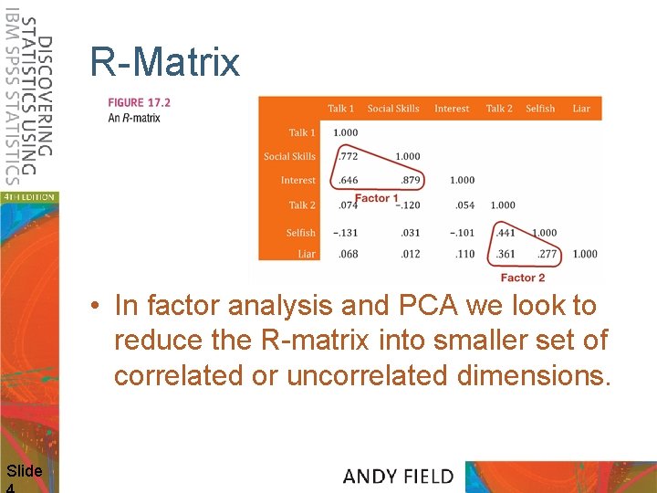
R-Matrix • In factor analysis and PCA we look to reduce the R-matrix into smaller set of correlated or uncorrelated dimensions. Slide

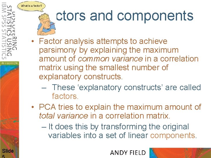
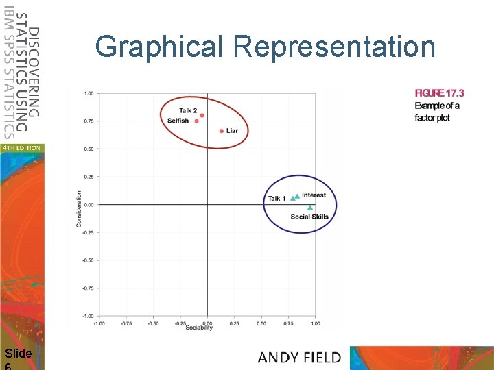
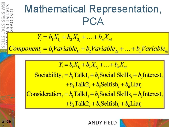
Factors and components • Factor analysis attempts to achieve parsimony by explaining the maximum amount of common variance in a correlation matrix using the smallest number of explanatory constructs. – These ‘explanatory constructs’ are called factors. • PCA tries to explain the maximum amount of total variance in a correlation matrix. – It does this by transforming the original variables into a set of linear components. Slide

Graphical Representation Slide

Mathematical Representation, PCA Slide

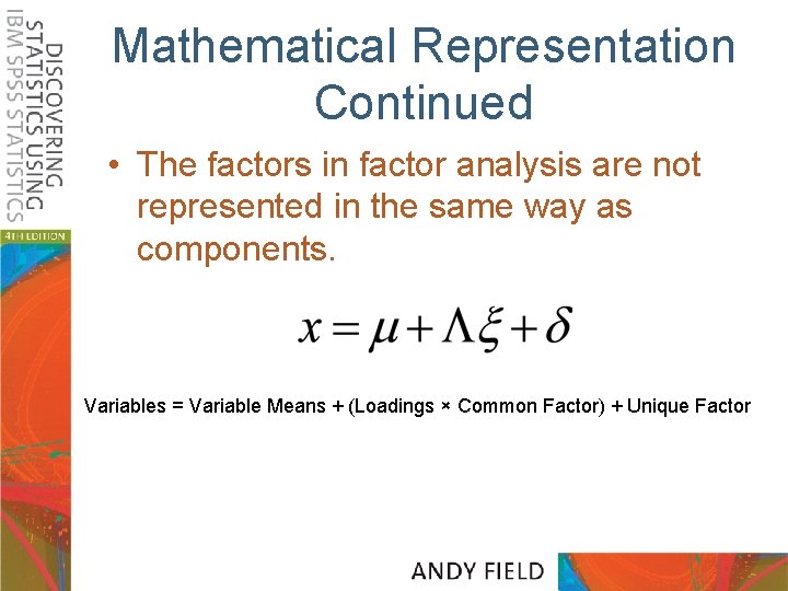
Mathematical Representation Continued • The factors in factor analysis are not represented in the same way as components. Variables = Variable Means + (Loadings × Common Factor) + Unique Factor

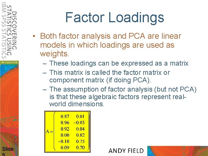
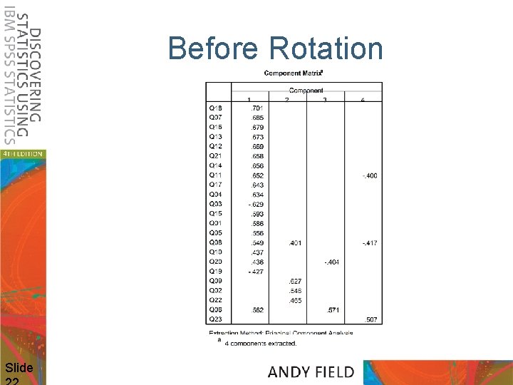
Factor Loadings • Both factor analysis and PCA are linear models in which loadings are used as weights. – These loadings can be expressed as a matrix – This matrix is called the factor matrix or component matrix (if doing PCA). – The assumption of factor analysis (but not PCA) is that these algebraic factors represent realworld dimensions. Slide

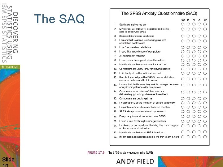
The SAQ Slide

Initial Considerations Slide • The quality of analysis depends upon the quality of the data (GI GO). • Test variables should correlate quite well – r >. 3. • Avoid Multicollinearity: – several variables highly correlated, r >. 80, tolerance >. 20. • Avoid Singularity: – some variables perfectly correlated, r = 1, tolerance = 0. • Screen the correlation matrix eliminate any variables that obviously cause concern. • Conduct multicollinearity analysis (as in multiple regression, but with case number as the dependent variable).

Further Considerations • Determinant: – Indicator of multicollinearity – should be greater than 0. 00001. • Kaiser-Meyer-Olkin (KMO): – Measures sampling adequacy – should be greater than 0. 5. • Bartlett’s Test of Sphericity: – Tests whether the R-matrix is an identity matrix – should be significant at p <. 05. • Anti-Image Matrix: – Measures of sampling adequacy on diagonal, – Off-diagonal elements should be small. • Reproduced: – Correlation matrix after rotation – most residuals should be < |0. 05| Slide

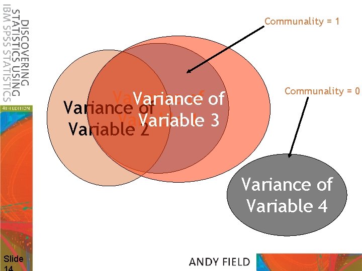
Finding Factors: Communality • Common Variance: – Variance that a variable shares with other variables. • Unique Variance: – Variance that is unique to a particular variable. • The proportion of common variance in a variable is called the communality. • Communality = 1, All variance shared. • Communality = 0, No variance shared. • 0 < Communality < 1 = Some variance shared. Slide

Communality = 1 Variance of of Variance of Variable 1 3 Variable 2 Communality = 0 Variance of Variable 4 Slide

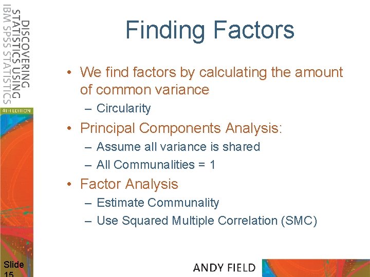
Finding Factors • We find factors by calculating the amount of common variance – Circularity • Principal Components Analysis: – Assume all variance is shared – All Communalities = 1 • Factor Analysis – Estimate Communality – Use Squared Multiple Correlation (SMC) Slide

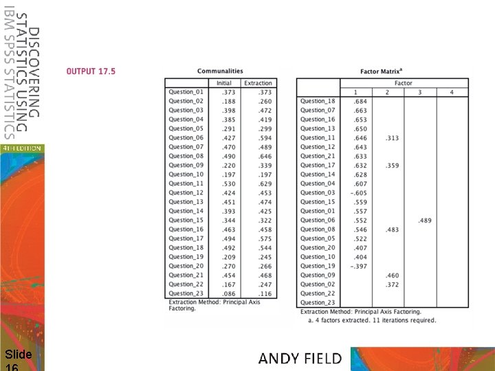
Slide

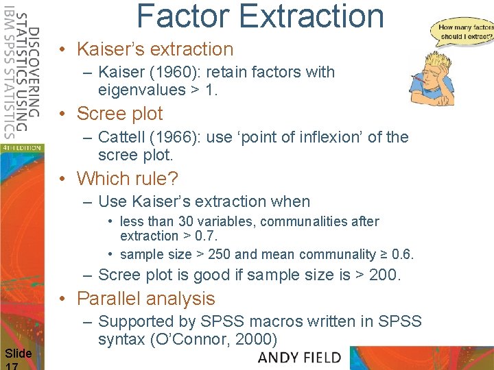
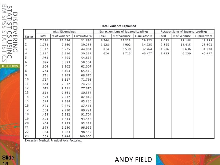
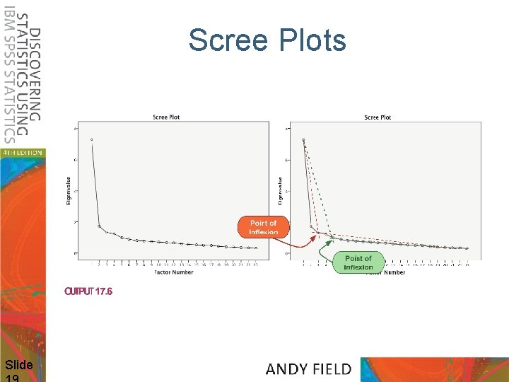
Factor Extraction • Kaiser’s extraction – Kaiser (1960): retain factors with eigenvalues > 1. • Scree plot – Cattell (1966): use ‘point of inflexion’ of the scree plot. • Which rule? – Use Kaiser’s extraction when • less than 30 variables, communalities after extraction > 0. 7. • sample size > 250 and mean communality ≥ 0. 6. – Scree plot is good if sample size is > 200. • Parallel analysis Slide – Supported by SPSS macros written in SPSS syntax (O’Connor, 2000)

Slide

Scree Plots Slide

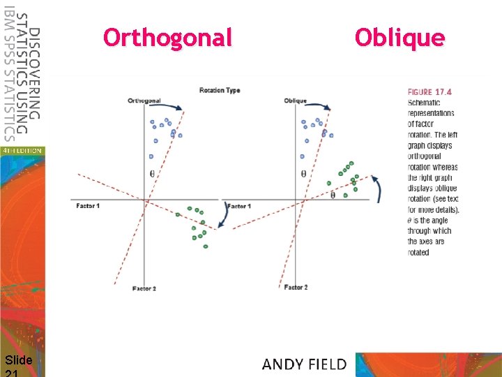
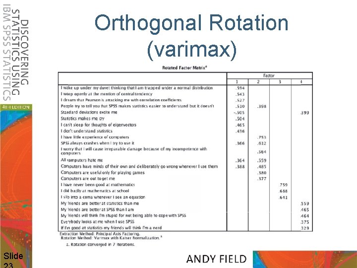
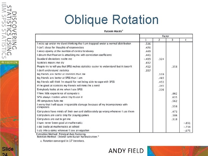
Rotation • To aid interpretation it is possible to maximise the loading of a variable on one factor while minimising its loading on all other factors • This is known as Factor Rotation • There are two types: – Orthogonal (factors are uncorrelated) – Oblique (factors intercorrelate) Slide

Orthogonal Slide Oblique

Before Rotation Slide

Orthogonal Rotation (varimax) Slide

Oblique Rotation Slide

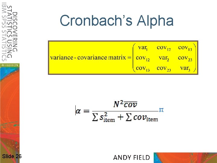
Reliability • Test-Retest Method – What about practice effects/mood states? • Alternate Form Method – Expensive and Impractical • Split-Half Method – Splits the questionnaire into two random halves, calculates scores and correlates them. • Cronbach’s alpha – Splits the questionnaire into all possible halves, calculates the scores, correlates them and averages the correlation for all splits (well, sort of …). – Ranges from 0 (no reliability) to 1 (complete reliability) Slide

Cronbach’s Alpha Slide 26

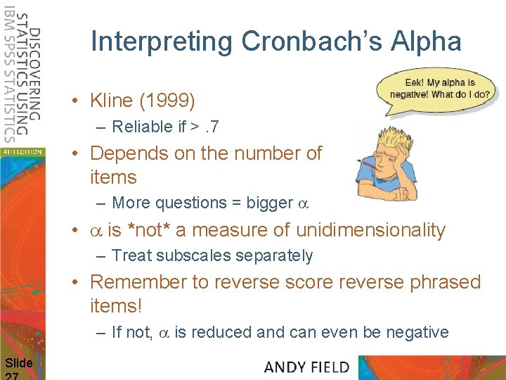
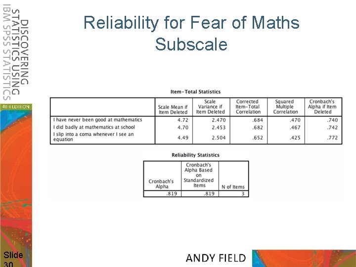
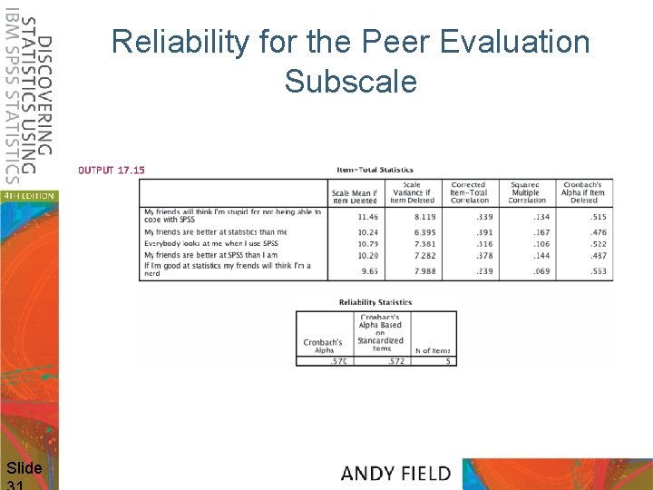
Interpreting Cronbach’s Alpha • Kline (1999) – Reliable if >. 7 • Depends on the number of items – More questions = bigger • is *not* a measure of unidimensionality – Treat subscales separately • Remember to reverse score reverse phrased items! – If not, is reduced and can even be negative Slide

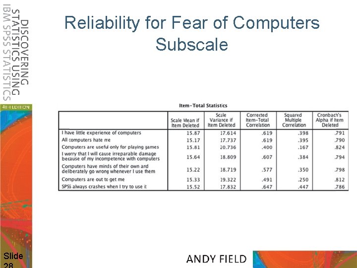
Reliability for Fear of Computers Subscale Slide

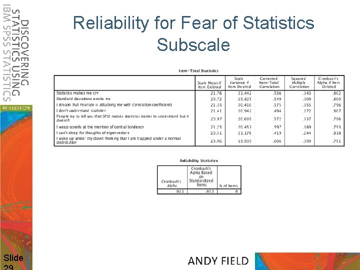
Reliability for Fear of Statistics Subscale Slide

Reliability for Fear of Maths Subscale Slide

Reliability for the Peer Evaluation Subscale Slide

The End? • Describe Factor Structure/Reliability • What items should be retained? – What items did you eliminate and why? • Application – Where will your questionnaire be used? – How does it fit in with psychological theory? Slide

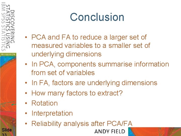
Conclusion Slide • PCA and FA to reduce a larger set of measured variables to a smaller set of underlying dimensions • In PCA, components summarise information from set of variables • In FA, factors are underlying dimensions • How many factors to extract? • Rotation • Interpretation • Reliability analysis after PCA/FA