Exploratory Data Analysis Exploratory Data Analysis EDA Descriptive

Exploratory Data Analysis

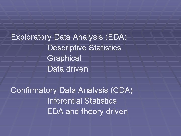
Exploratory Data Analysis (EDA) Descriptive Statistics Graphical Data driven Confirmatory Data Analysis (CDA) Inferential Statistics EDA and theory driven

Before you begin your analyses, it is imperative that you examine all your variables. Why? To listen to the data: -to catch mistakes -to see patterns in the data -to find violations of statistical assumptions …and because if you don’t, you will have trouble later

Overview Part I: The Basics or “I got mean and deviant and now I’m considered normal” Part II: Exploratory Data Analysis or “I ask Skew how to recover from kurtosis and only hear ‘Get out, liar!’”

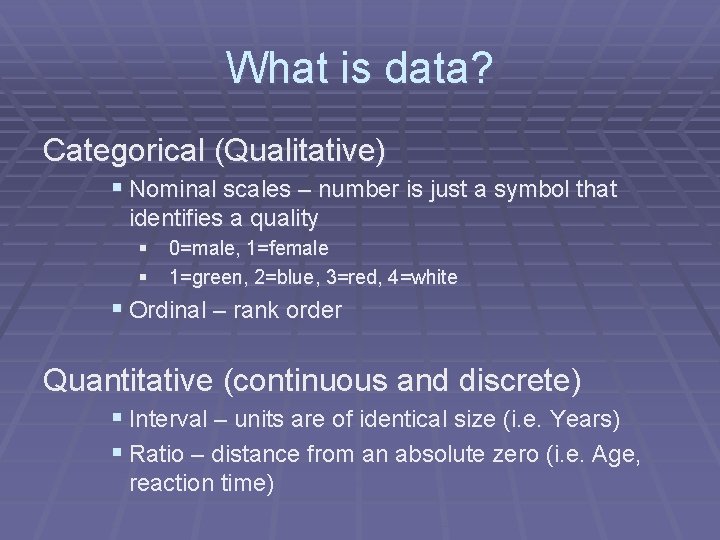
What is data? Categorical (Qualitative) § Nominal scales – number is just a symbol that identifies a quality § § 0=male, 1=female 1=green, 2=blue, 3=red, 4=white § Ordinal – rank order Quantitative (continuous and discrete) § Interval – units are of identical size (i. e. Years) § Ratio – distance from an absolute zero (i. e. Age, reaction time)

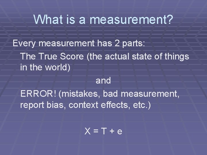
What is a measurement? Every measurement has 2 parts: The True Score (the actual state of things in the world) and ERROR! (mistakes, bad measurement, report bias, context effects, etc. ) X=T+e

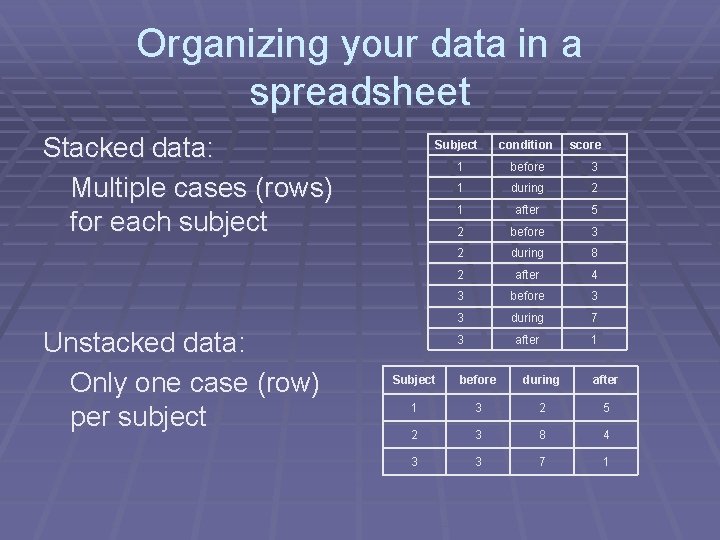
Organizing your data in a spreadsheet Stacked data: Multiple cases (rows) for each subject Unstacked data: Only one case (row) per subject Subject condition score 1 before 3 1 during 2 1 after 5 2 before 3 2 during 8 2 after 4 3 before 3 3 during 7 3 after 1 Subject before during after 1 3 2 5 2 3 8 4 3 3 7 1

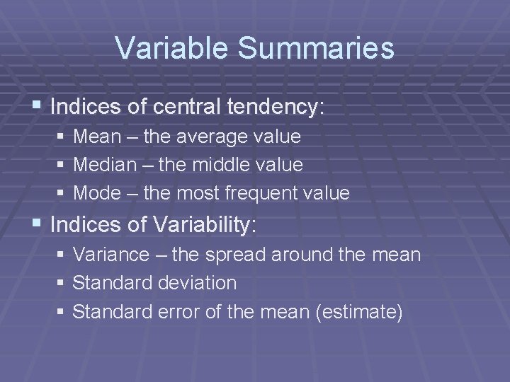
Variable Summaries § Indices of central tendency: § Mean – the average value § Median – the middle value § Mode – the most frequent value § Indices of Variability: § Variance – the spread around the mean § Standard deviation § Standard error of the mean (estimate)

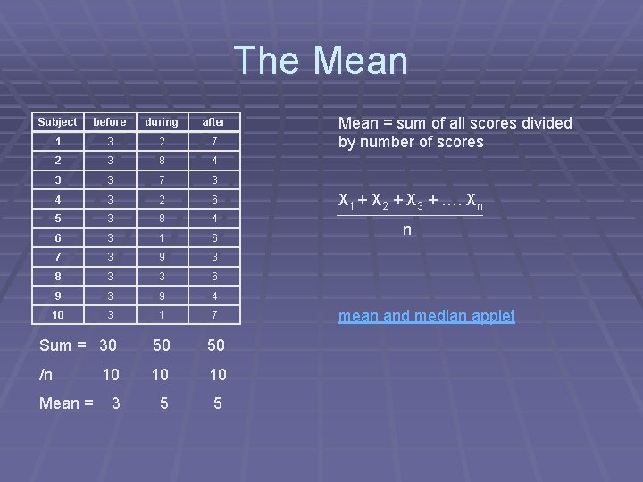
The Mean Subject before during after 1 3 2 7 2 3 8 4 3 3 7 3 4 3 2 6 5 3 8 4 6 3 1 6 7 3 9 3 8 3 3 6 9 3 9 4 10 3 1 7 Sum = 30 50 50 /n 10 10 10 3 5 5 Mean = sum of all scores divided by number of scores X 1 + X 2 + X 3 + …. Xn n mean and median applet

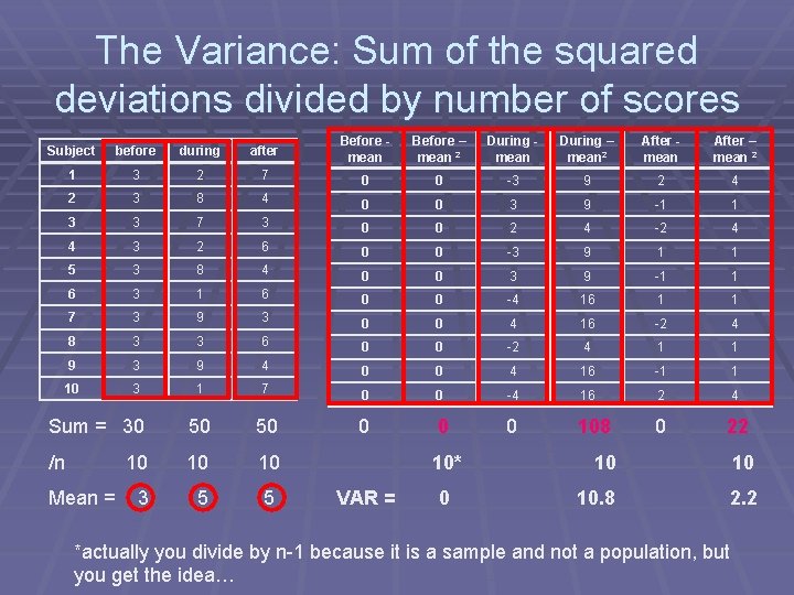
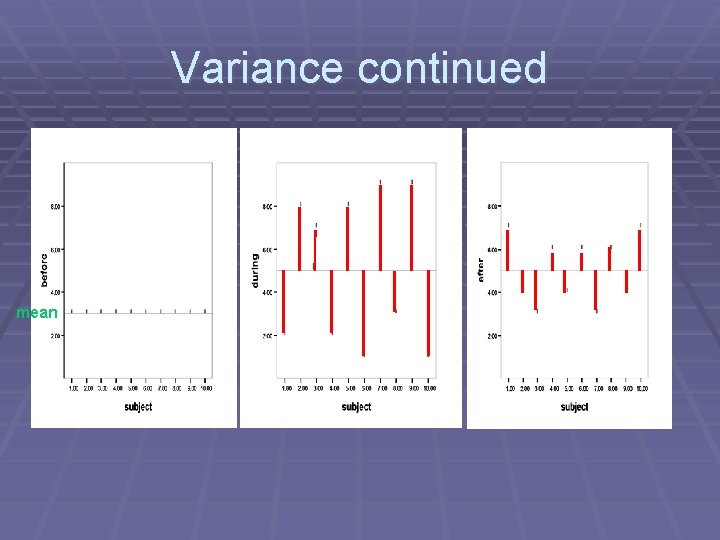
The Variance: Sum of the squared deviations divided by number of scores Subject before during after Before mean Before – mean 2 During mean During – mean 2 After mean After – mean 2 1 3 2 7 0 0 -3 9 2 4 2 3 8 4 0 0 3 9 -1 1 3 3 7 3 0 0 2 4 -2 4 4 3 2 6 0 0 -3 9 1 1 5 3 8 4 0 0 3 9 -1 1 6 3 1 6 0 0 -4 16 1 1 7 3 9 3 0 0 4 16 -2 4 8 3 3 6 0 0 -2 4 1 1 9 3 9 4 0 0 4 16 -1 1 10 3 1 7 0 0 -4 16 2 4 Sum = 30 50 50 0 108 0 22 /n 10 10 10 3 5 5 Mean = 10* VAR = 0 10 10 10. 8 2. 2 *actually you divide by n-1 because it is a sample and not a population, but you get the idea…

Variance continued mean

Distribution § Means and variances are ways to describe a distribution of scores. § Knowing about your distributions is one of the best ways to understand your data § A NORMAL (aka Gaussian) distribution is the most common assumption of statistics, thus it is often important to check if your data are normally distributed. Normal Distribution applet normaldemo. html sorry, these don’t work yet

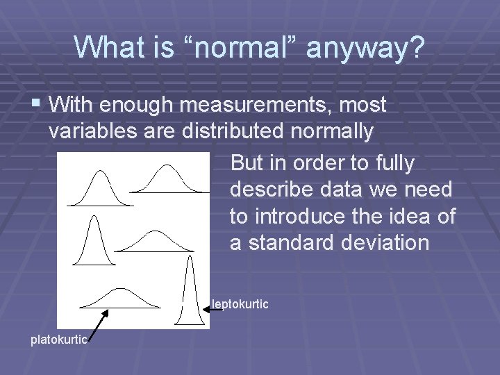
What is “normal” anyway? § With enough measurements, most variables are distributed normally But in order to fully describe data we need to introduce the idea of a standard deviation leptokurtic platokurtic

Standard deviation Variance, as calculated earlier, is arbitrary. What does it mean to have a variance of 10. 8? Or 2. 2? Or 1459. 092? Or 0. 000001? Nothing. But if you could “standardize” that value, you could talk about any variance (i. e. deviation) in equivalent terms. Standard Deviations are simply the square root of the variance

Standard deviation The process of standardizing deviations goes like this: 1. Score (in the units that are meaningful) 2. Mean 3. Each score’s deviation from the mean 4. Square that deviation 5. Sum all the squared deviations (Sum of Squares) 6. Divide by n (if population) or n-1 (if sample) 7. Square root – now the value is in the units we started with!!!

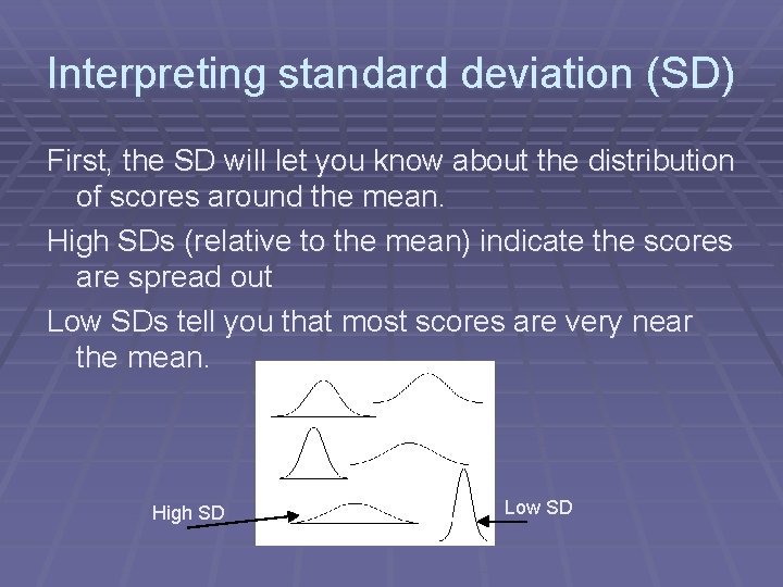
Interpreting standard deviation (SD) First, the SD will let you know about the distribution of scores around the mean. High SDs (relative to the mean) indicate the scores are spread out Low SDs tell you that most scores are very near the mean. High SD Low SD

Interpreting standard deviation (SD) Second, you can then interpret any individual score in terms of the SD. For example: mean = 50, SD = 10 versus mean = 50, SD = 1 A score of 55 is: 0. 5 Standard deviation units from the mean (not much) OR 5 standard deviation units from mean (a lot!)

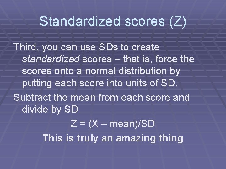
Standardized scores (Z) Third, you can use SDs to create standardized scores – that is, force the scores onto a normal distribution by putting each score into units of SD. Subtract the mean from each score and divide by SD Z = (X – mean)/SD This is truly an amazing thing

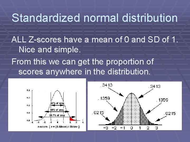
Standardized normal distribution ALL Z-scores have a mean of 0 and SD of 1. Nice and simple. From this we can get the proportion of scores anywhere in the distribution.

The trouble with normal We violate assumptions about statistical tests if the distributions of our variables are not approximately normal. Thus, we must first examine each variable’s distribution and make adjustments when necessary so that assumptions are met. sample mean applet not working yet

Part II Examine every variable for: Out of range values Normality Outliers

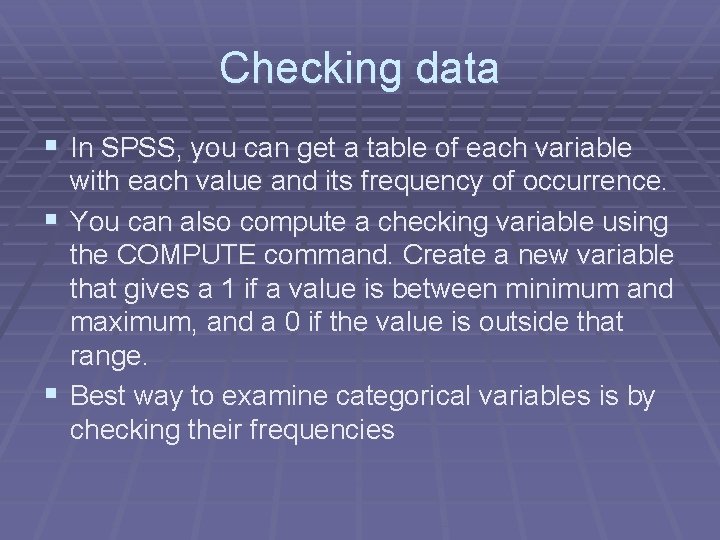
Checking data § In SPSS, you can get a table of each variable with each value and its frequency of occurrence. § You can also compute a checking variable using the COMPUTE command. Create a new variable that gives a 1 if a value is between minimum and maximum, and a 0 if the value is outside that range. § Best way to examine categorical variables is by checking their frequencies

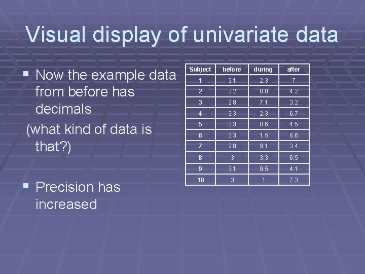
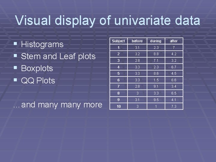
Visual display of univariate data § Now the example data from before has decimals (what kind of data is that? ) § Precision has increased Subject before during after 1 3. 1 2. 3 7 2 3. 2 8. 8 4. 2 3 2. 8 7. 1 3. 2 4 3. 3 2. 3 6. 7 5 3. 3 8. 6 4. 5 6 3. 3 1. 5 6. 6 7 2. 8 9. 1 3. 4 8 3 3. 3 6. 5 9 3. 1 9. 5 4. 1 10 3 1 7. 3

Visual display of univariate data § § Histograms Stem and Leaf plots Boxplots QQ Plots …and many more Subject before during after 1 3. 1 2. 3 7 2 3. 2 8. 8 4. 2 3 2. 8 7. 1 3. 2 4 3. 3 2. 3 6. 7 5 3. 3 8. 6 4. 5 6 3. 3 1. 5 6. 6 7 2. 8 9. 1 3. 4 8 3 3. 3 6. 5 9 3. 1 9. 5 4. 1 10 3 1 7. 3

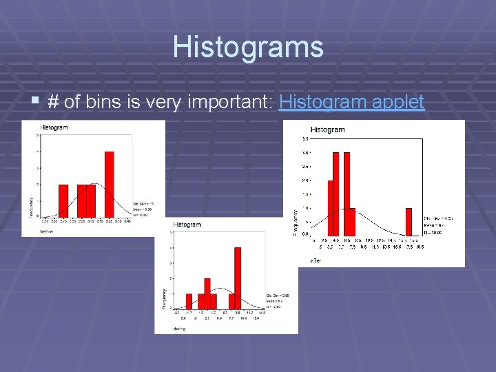
Histograms § # of bins is very important: Histogram applet

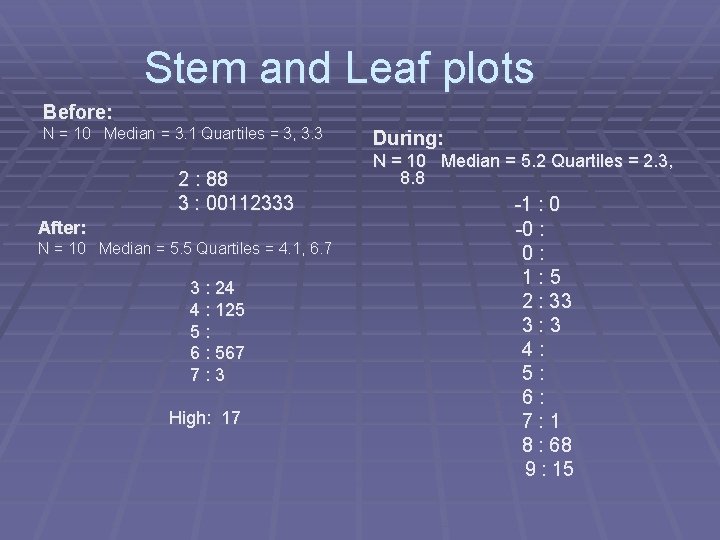
Stem and Leaf plots Before: N = 10 Median = 3. 1 Quartiles = 3, 3. 3 2 : 88 3 : 00112333 After: N = 10 Median = 5. 5 Quartiles = 4. 1, 6. 7 3 : 24 4 : 125 5: 6 : 567 7: 3 High: 17 During: N = 10 Median = 5. 2 Quartiles = 2. 3, 8. 8 -1 : 0 -0 : 0: 1: 5 2 : 33 3: 3 4: 5: 6: 7: 1 8 : 68 9 : 15

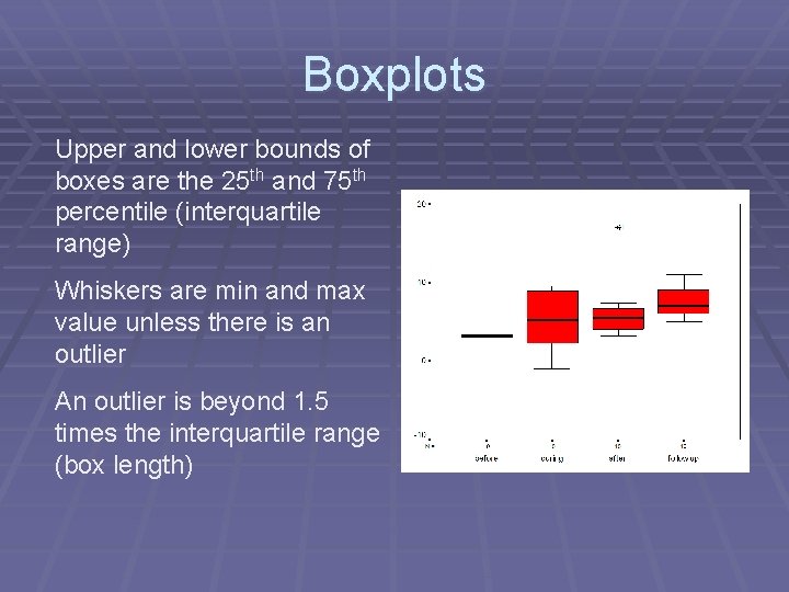
Boxplots Upper and lower bounds of boxes are the 25 th and 75 th percentile (interquartile range) Whiskers are min and max value unless there is an outlier An outlier is beyond 1. 5 times the interquartile range (box length)

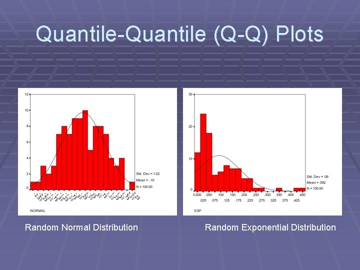
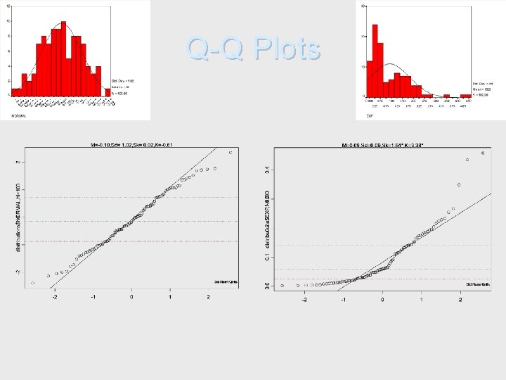
Quantile-Quantile (Q-Q) Plots Random Normal Distribution Random Exponential Distribution

Q-Q Plots

So…what do you do? If you find a mistake, fix it. If you find an outlier, trim it or delete it. If your distributions are askew, transform the data.

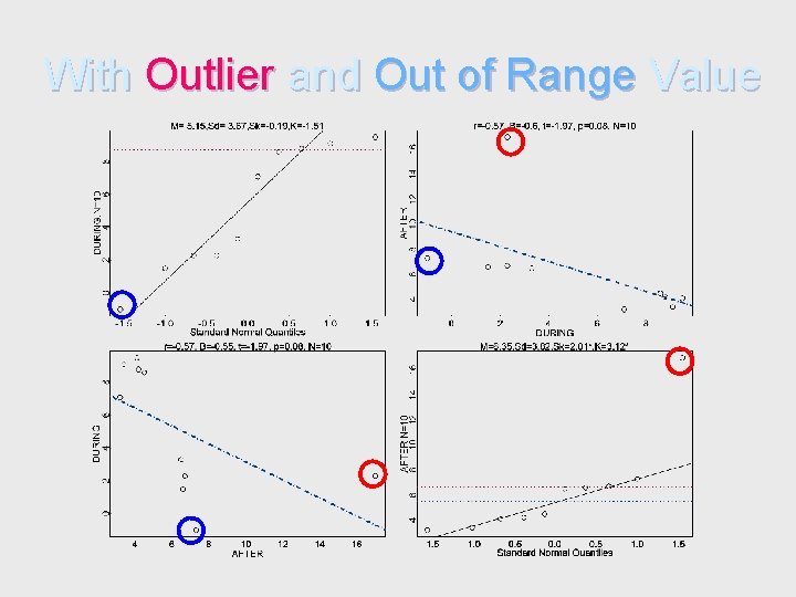
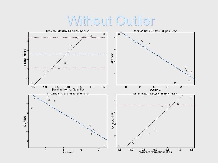
Dealing with Outliers First, try to explain it. In a normal distribution 0. 4% are outliers (>2. 7 SD) and 1 in a million is an extreme outlier (>4. 72 SD). For analyses you can: Delete the value – crude but effective Change the outlier to value ~3 SD from mean “Winsorize” it (make = to next highest value) “Trim” the mean – recalculate mean from data within interquartile range

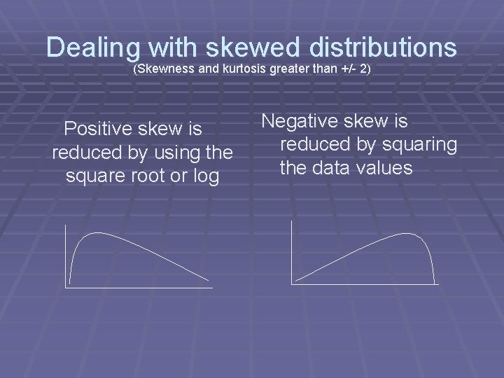
Dealing with skewed distributions (Skewness and kurtosis greater than +/- 2) Positive skew is reduced by using the square root or log Negative skew is reduced by squaring the data values

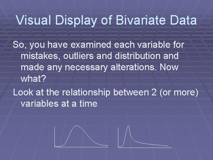
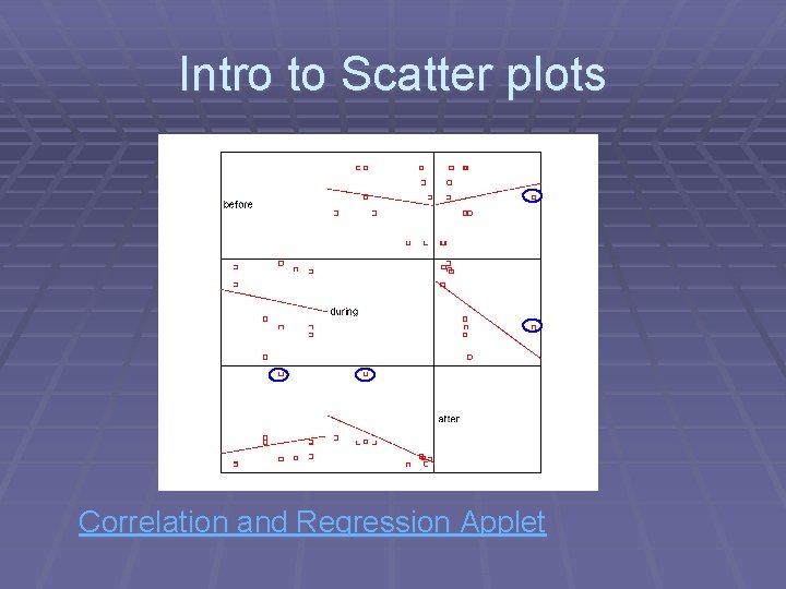
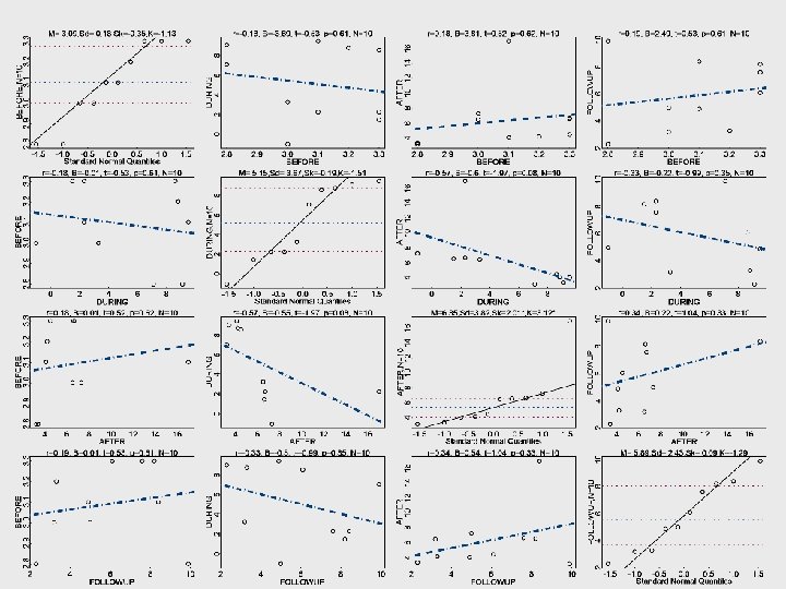
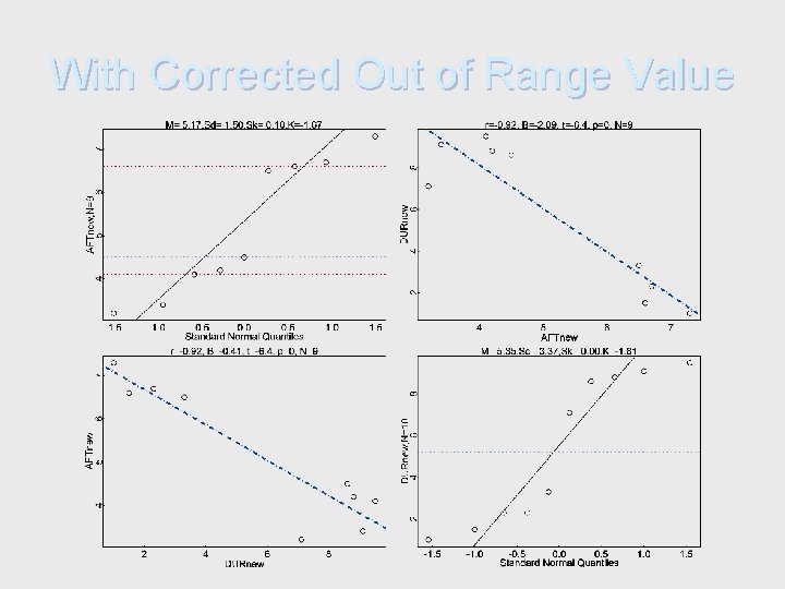
Visual Display of Bivariate Data So, you have examined each variable for mistakes, outliers and distribution and made any necessary alterations. Now what? Look at the relationship between 2 (or more) variables at a time

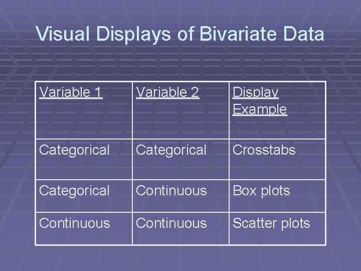
Visual Displays of Bivariate Data Variable 1 Variable 2 Display Example Categorical Crosstabs Categorical Continuous Box plots Continuous Scatter plots

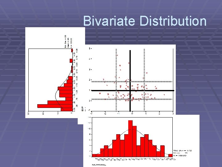
Bivariate Distribution

Intro to Scatter plots Correlation and Regression Applet

With Outlier and Out of Range Value

Without Outlier

With Corrected Out of Range Value

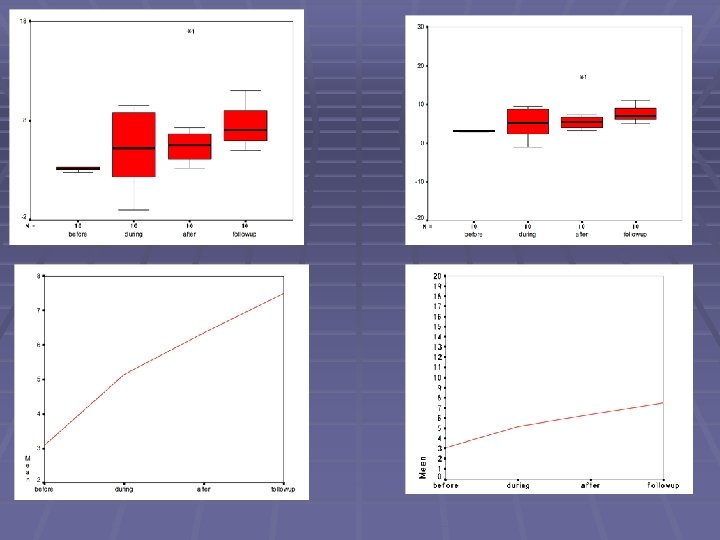
Scales of Graphs § It is very important to pay attention to the scale that you are using when you are plotting. § Compare the following graphs created from identical data

Summary § Examine all your variables thoroughly and carefully before you begin analysis § Use visual displays whenever possible § Transform each variable as necessary to deal with mistakes, outliers, and distributions

Resources on line http: //www. statsoftinc. com/textbook/stathome. html http: //www. cs. uni. edu/~campbell/stat/lectures. html http: //www. psychstat. smsu. edu/sbk 00. htm http: //davidmlane. com/hyperstat/ http: //bcs. whfreeman. com/ips 4 e/pages/bcs-main. asp? v=category&s=00010&n=99000&i=99010. 01&o= http: //trochim. human. cornell. edu/selstat/ssstart. htm http: //www. math. yorku. ca/SCS/Stat. Resource. html#Data. Vis

Recommended Reading § Anything by Tukey, especially Exploratory Data Analysis (Tukey, 1997) § Anything by Cleveland, especially Visualizing Data (Cleveland, 1993) § Visual Display of Quantitative Information (Tufte, 1983) § Anything on statistics by Jacob Cohen or Paul Meehl.

for next time § http: //www. execpc. com/~helberg/pitfalls