Recurrent Neural Networks Learning Extension and Applications Ting

Recurrent Neural Networks - Learning, Extension and Applications Ting Chen Nov. 20, 2015 Courtesy to all the sources of materials used in this slides. Especially to Geff. Hinton, whose slides I based on.

Sequence modeling Review • Section overview – Memoryless models – Models with memory • Linear Dynamical Systems • Hidden Markov Models • Recurrent Neural Networks: architecture

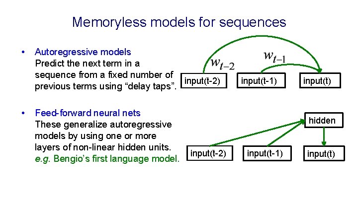
Memoryless models for sequences • • Autoregressive models Predict the next term in a sequence from a fixed number of input(t-2) previous terms using “delay taps”. Feed-forward neural nets These generalize autoregressive models by using one or more layers of non-linear hidden units. e. g. Bengio’s first language model. input(t-1) input(t) hidden input(t-2) input(t-1) input(t)

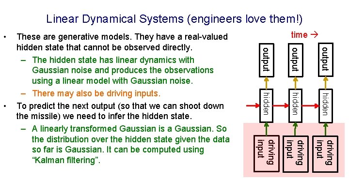
Linear Dynamical Systems (engineers love them!) • time output hidden driving input • These are generative models. They have a real-valued hidden state that cannot be observed directly. – The hidden state has linear dynamics with Gaussian noise and produces the observations using a linear model with Gaussian noise. – There may also be driving inputs. To predict the next output (so that we can shoot down the missile) we need to infer the hidden state. – A linearly transformed Gaussian is a Gaussian. So the distribution over the hidden state given the data so far is Gaussian. It can be computed using “Kalman filtering”.

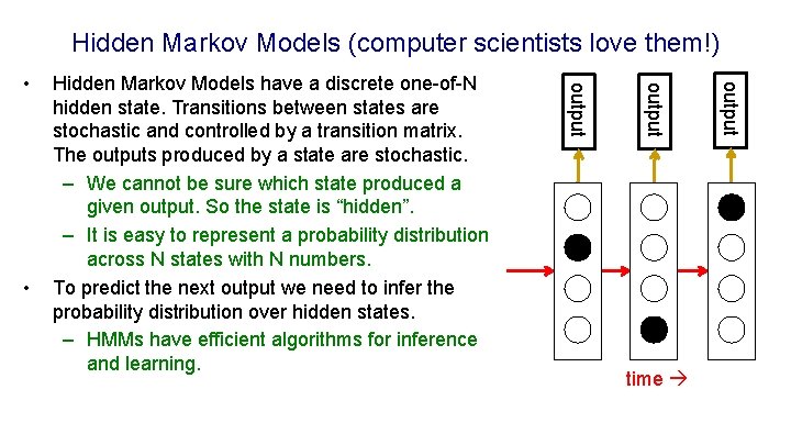
Hidden Markov Models (computer scientists love them!) time output • Hidden Markov Models have a discrete one-of-N hidden state. Transitions between states are stochastic and controlled by a transition matrix. The outputs produced by a state are stochastic. – We cannot be sure which state produced a given output. So the state is “hidden”. – It is easy to represent a probability distribution across N states with N numbers. To predict the next output we need to infer the probability distribution over hidden states. – HMMs have efficient algorithms for inference and learning. output •

A fundamental limitation of HMMs • • • Consider what happens when a hidden Markov model generates data. – At each time step it must select one of its hidden states. So with N hidden states it can only remember log(N) bits about what it generated so far. Consider the information that the first half of an utterance contains about the second half: – The syntax needs to fit (e. g. number and tense agreement). – The semantics needs to fit. The intonation needs to fit. – The accent, rate, volume, and vocal tract characteristics must all fit. All these aspects combined could be 100 bits of information that the first half of an utterance needs to convey to the second half. 2^100 is big!

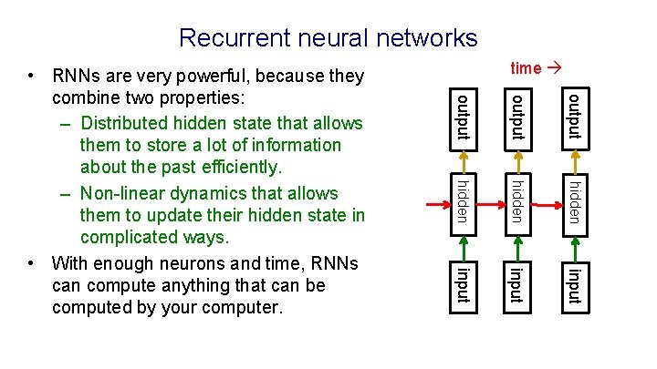
Recurrent neural networks time output hidden input • RNNs are very powerful, because they combine two properties: – Distributed hidden state that allows them to store a lot of information about the past efficiently. – Non-linear dynamics that allows them to update their hidden state in complicated ways. • With enough neurons and time, RNNs can compute anything that can be computed by your computer.

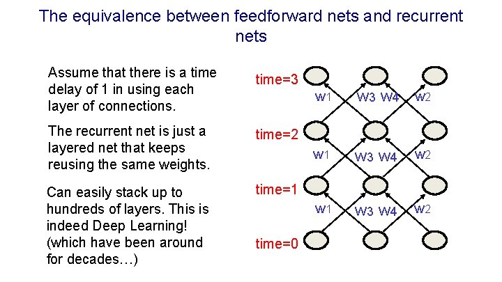
The equivalence between feedforward nets and recurrent nets Assume that there is a time delay of 1 in using each layer of connections. time=3 The recurrent net is just a layered net that keeps reusing the same weights. time=2 Can easily stack up to hundreds of layers. This is indeed Deep Learning! (which have been around for decades…) time=1 w 1 w w 3 w 4 2 w 1 w 2 w 3 w 4 time=0

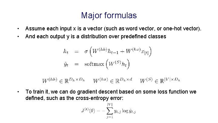
Major formulas • • Assume each input x is a vector (such as word vector, or one-hot vector). And each output y is a distribution over predefined classes • To train it, we can do gradient descent based on some loss function we defined, such as the cross-entropy error:

An irritating extra issue • We need to specify the initial activity state of all the hidden and output units. • We could just fix these initial states to have some default value like 0. 5. • But it is better to treat the initial states as learned parameters. • We learn them in the same way as we learn the weights. – Start off with an initial random guess for the initial states. – At the end of each training sequence, backpropagate through time all the way to the initial states to get the gradient of the error function with respect to each initial state. – Adjust the initial states by following the negative gradient.

Training RNNs with backpropagation • Section Overview – Backpropagation Through Time (BPTT) – Vanishing/Exploding gradients • Why you care? • Why it happens? • How to fix it?

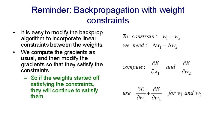
Reminder: Backpropagation with weight constraints • • It is easy to modify the backprop algorithm to incorporate linear constraints between the weights. We compute the gradients as usual, and then modify the gradients so that they satisfy the constraints. – So if the weights started off satisfying the constraints, they will continue to satisfy them.

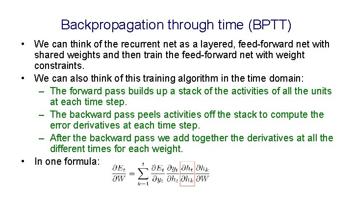
Backpropagation through time (BPTT) • We can think of the recurrent net as a layered, feed-forward net with shared weights and then train the feed-forward net with weight constraints. • We can also think of this training algorithm in the time domain: – The forward pass builds up a stack of the activities of all the units at each time step. – The backward pass peels activities off the stack to compute the error derivatives at each time step. – After the backward pass we add together the derivatives at all the different times for each weight. • In one formula:

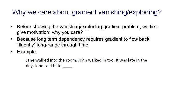
Why we care about gradient vanishing/exploding? • Before showing the vanishing/exploding gradient problem, we first give motivation: why you care? • Because long term dependency requires gradient to flow back “fluently” long-range through time • Example:

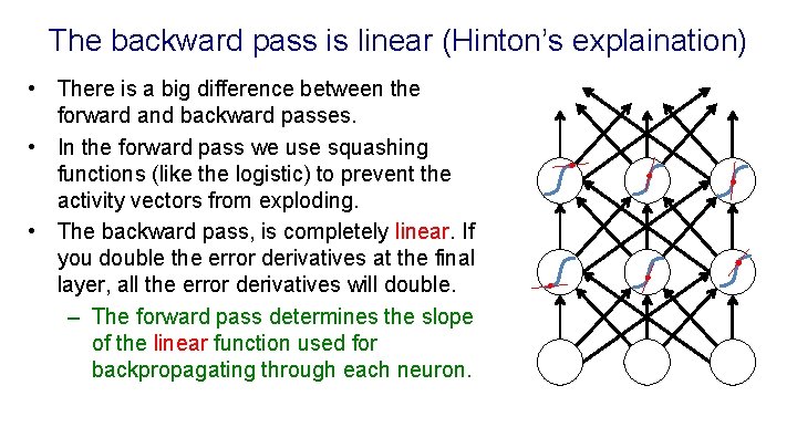
The backward pass is linear (Hinton’s explaination) • There is a big difference between the forward and backward passes. • In the forward pass we use squashing functions (like the logistic) to prevent the activity vectors from exploding. • The backward pass, is completely linear. If you double the error derivatives at the final layer, all the error derivatives will double. – The forward pass determines the slope of the linear function used for backpropagating through each neuron.

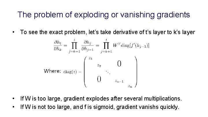
The problem of exploding or vanishing gradients • To see the exact problem, let’s take derivative of t’s layer to k’s layer • If W is too large, gradient explodes after several multiplications. • If W is not too large, and f is sigmoid, gradient vanishs quickly.

Four effective ways to learn an RNN • • Long Short Term Memory • Make the RNN out of little modules that are designed to remember values for a long time. Hessian Free Optimization: Deal with the vanishing gradients problem by using a fancy optimizer that can detect directions with a tiny gradient but • even smaller curvature. – The HF optimizer ( Martens & Sutskever, 2011) is good at this. Echo State Networks: Initialize the input hidden and output hidden connections very carefully so that the hidden state has a huge reservoir of weakly coupled oscillators which can be selectively driven by the input. – ESNs only need to learn the hidden output connections. Good initialization with momentum Initialize like in Echo State Networks, but then learn all of the connections using momentum.

An (super hip) extension of standard RNNs • Section overview – Long Short-Term Memory (LSTM) • Intuition • Formulation

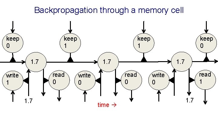
Long Short Term Memory (LSTM) • Hochreiter & Schmidhuber (1997) solved the problem of getting an RNN to remember things for a long time (like hundreds of time steps). • They designed a memory cell using logistic and linear units with multiplicative interactions. • Information gets into the cell whenever its “write” gate is on. • The information stays in the cell so long as its “keep” gate is on. • Information can be read from the cell by turning on its “read” gate.

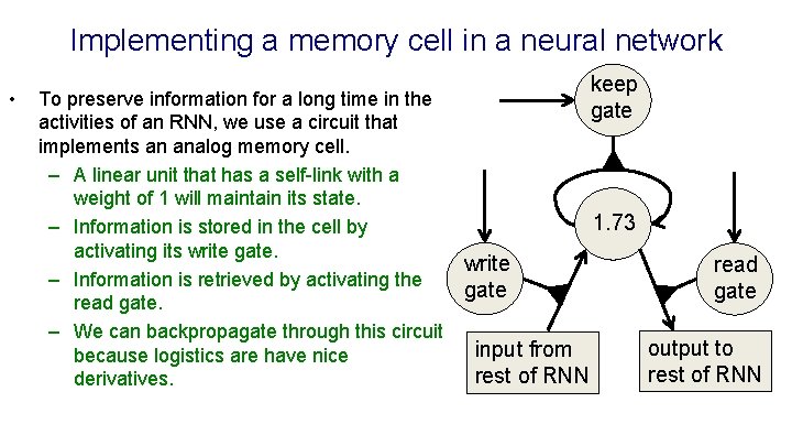
Implementing a memory cell in a neural network • keep To preserve information for a long time in the gate activities of an RNN, we use a circuit that implements an analog memory cell. – A linear unit that has a self-link with a weight of 1 will maintain its state. 1. 73 – Information is stored in the cell by activating its write gate. write read – Information is retrieved by activating the gate read gate. – We can backpropagate through this circuit output to input from because logistics are have nice rest of RNN derivatives.

Backpropagation through a memory cell keep 0 keep 1 1. 7 write 1 1. 7 read 0 write 0 time keep 0 read 1 write 0 1. 7

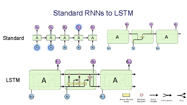
Standard RNNs to LSTM Standard LSTM

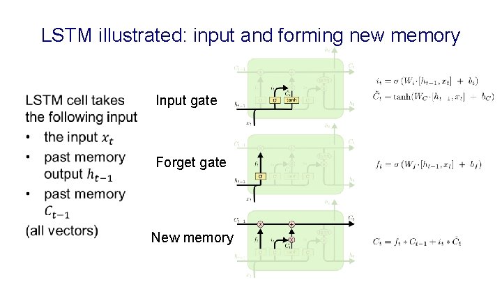
LSTM illustrated: input and forming new memory Input gate Forget gate New memory

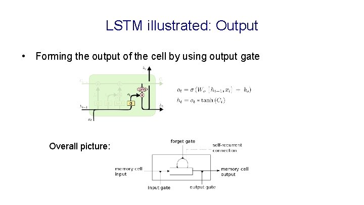
LSTM illustrated: Output • Forming the output of the cell by using output gate Overall picture:

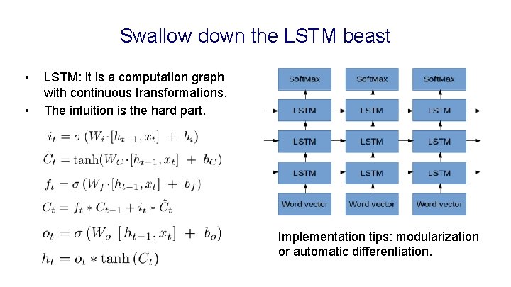
Swallow down the LSTM beast • • LSTM: it is a computation graph with continuous transformations. The intuition is the hard part. Implementation tips: modularization or automatic differentiation.

(NLP) Applications of RNNs • Section overview – Sentiment analysis / text classification – Machine translation and conversation modeling – Sentence skip-thought vectors NLP is kind of like a rabbit in the headlights of the deep learning machine. - Neil Lawrence, DL workshop panel, 2015

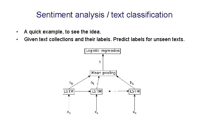
Sentiment analysis / text classification • • A quick example, to see the idea. Given text collections and their labels. Predict labels for unseen texts.

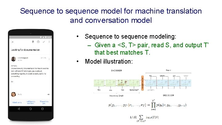
Sequence to sequence model for machine translation and conversation model • Sequence to sequence modeling: – Given a <S, T> pair, read S, and output T’ that best matches T. • Model illustration:

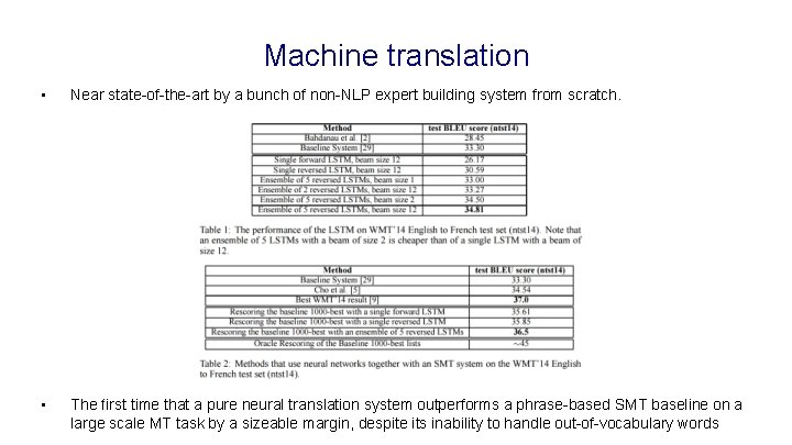
Machine translation • Near state-of-the-art by a bunch of non-NLP expert building system from scratch. • The first time that a pure neural translation system outperforms a phrase-based SMT baseline on a large scale MT task by a sizeable margin, despite its inability to handle out-of-vocabulary words

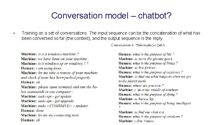
Conversation model – chatbot? • Training on a set of conversations. The input sequence can be the concatenation of what has been conversed so far (the context), and the output sequence is the reply.

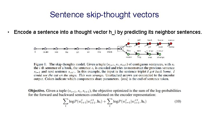
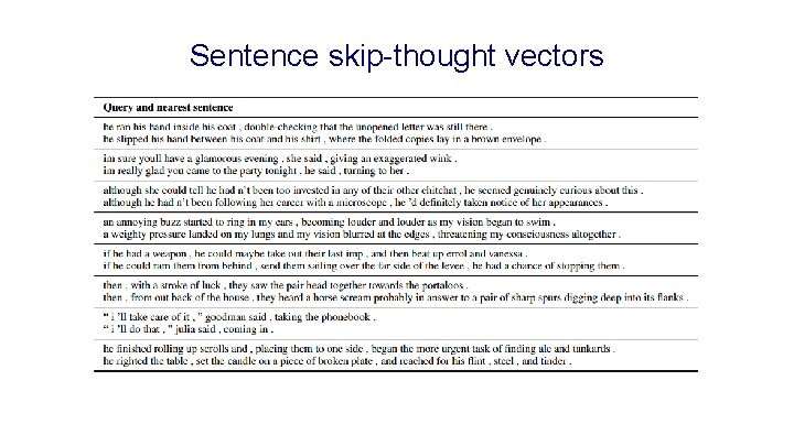
Sentence skip-thought vectors • Encode a sentence into a thought vector h_i by predicting its neighbor sentences.

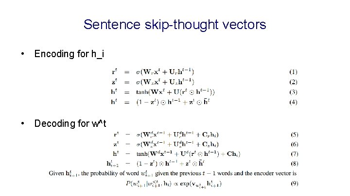
Sentence skip-thought vectors • Encoding for h_i • Decoding for w^t

Sentence skip-thought vectors