Recommendation and Advertising Shannon Quinn with thanks to

Recommendation and Advertising Shannon Quinn (with thanks to J. Leskovec, A. Rajaraman, and J. Ullman of Stanford University)

Lecture breakdown • Part 1: Advertising – Bipartite Matching – Ad. Words • Part 2: Recommendation – Collaborative Filtering – Latent Factor Models

1: Advertising on the Web

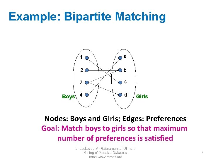
Example: Bipartite Matching 1 a 2 b 3 c Boys 4 d Girls Nodes: Boys and Girls; Edges: Preferences Goal: Match boys to girls so that maximum number of preferences is satisfied J. Leskovec, A. Rajaraman, J. Ullman: Mining of Massive Datasets, 4

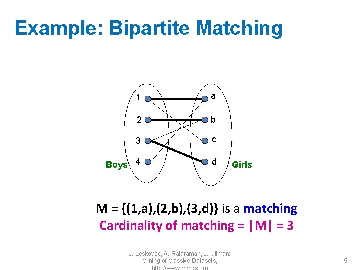
Example: Bipartite Matching 1 a 2 b 3 c Boys 4 d Girls M = {(1, a), (2, b), (3, d)} is a matching Cardinality of matching = |M| = 3 J. Leskovec, A. Rajaraman, J. Ullman: Mining of Massive Datasets, 5

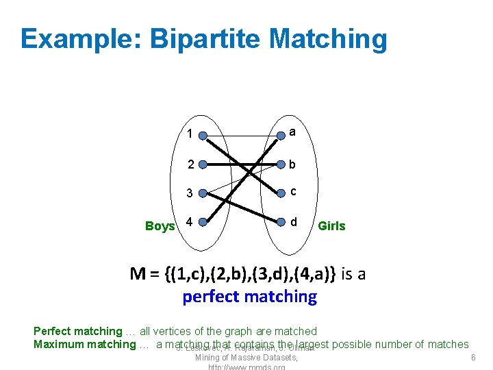
Example: Bipartite Matching 1 a 2 b 3 c Boys 4 d Girls M = {(1, c), (2, b), (3, d), (4, a)} is a perfect matching Perfect matching … all vertices of the graph are matched Maximum matching … a matching that largest possible number of matches J. Leskovec, A. contains Rajaraman, the J. Ullman: Mining of Massive Datasets, 6

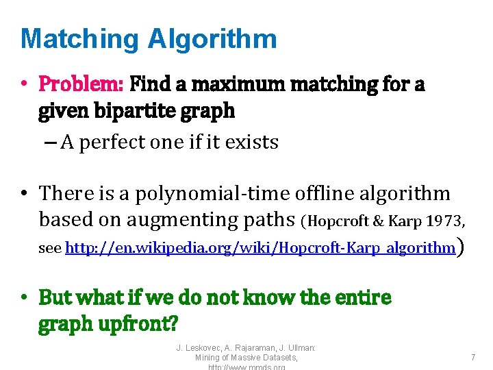
Matching Algorithm • Problem: Find a maximum matching for a given bipartite graph – A perfect one if it exists • There is a polynomial-time offline algorithm based on augmenting paths (Hopcroft & Karp 1973, see http: //en. wikipedia. org/wiki/Hopcroft-Karp_algorithm) • But what if we do not know the entire graph upfront? J. Leskovec, A. Rajaraman, J. Ullman: Mining of Massive Datasets, 7

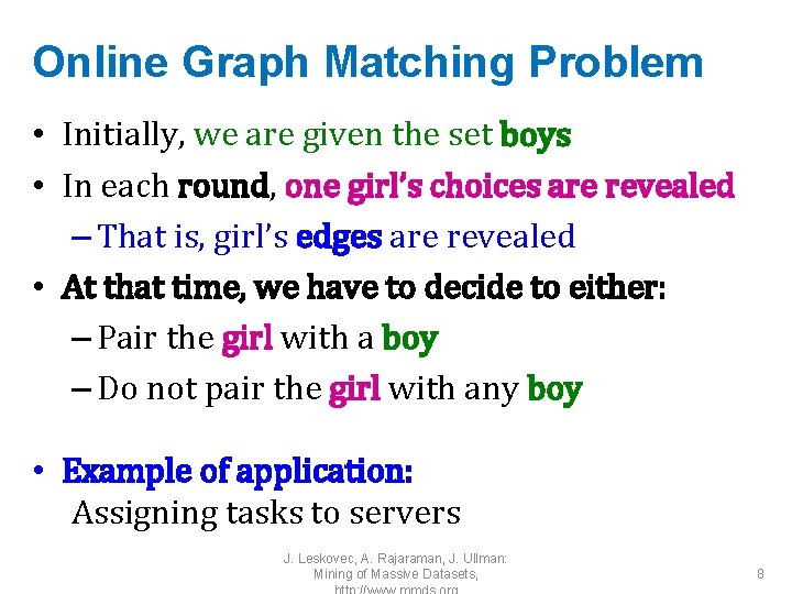
Online Graph Matching Problem • Initially, we are given the set boys • In each round, one girl’s choices are revealed – That is, girl’s edges are revealed • At that time, we have to decide to either: – Pair the girl with a boy – Do not pair the girl with any boy • Example of application: Assigning tasks to servers J. Leskovec, A. Rajaraman, J. Ullman: Mining of Massive Datasets, 8

Greedy Algorithm • Greedy algorithm for the online graph matching problem: – Pair the new girl with any eligible boy • If there is none, do not pair girl • How good is the algorithm? J. Leskovec, A. Rajaraman, J. Ullman: Mining of Massive Datasets, 9

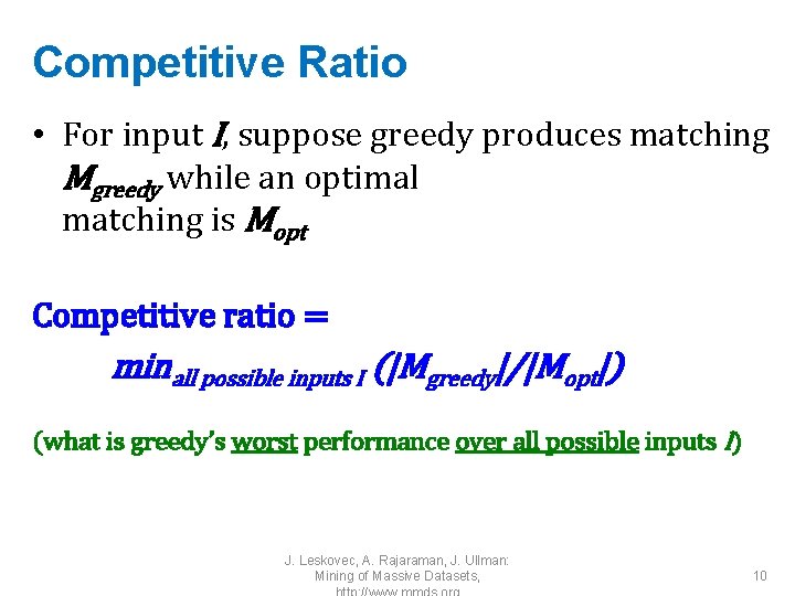
Competitive Ratio • For input I, suppose greedy produces matching Mgreedy while an optimal matching is Mopt Competitive ratio = minall possible inputs I (|Mgreedy|/|Mopt|) (what is greedy’s worst performance over all possible inputs I) J. Leskovec, A. Rajaraman, J. Ullman: Mining of Massive Datasets, 10

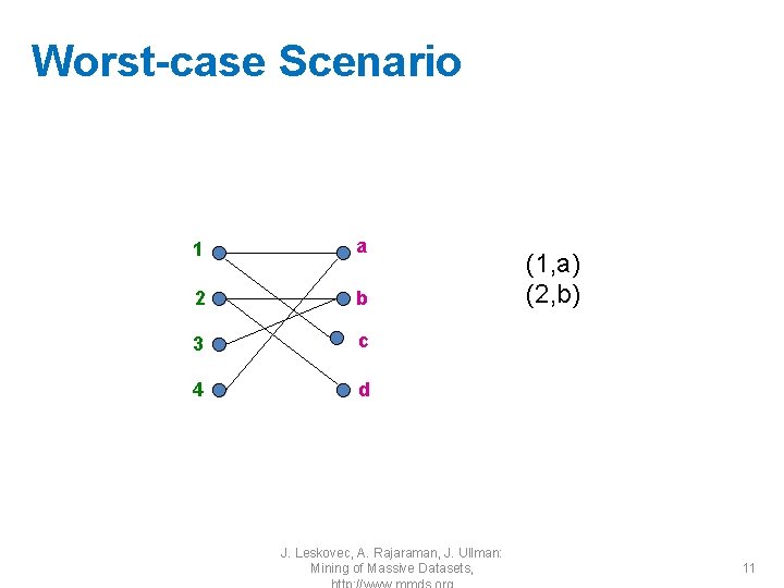
Worst-case Scenario 1 a 2 b 3 c 4 d J. Leskovec, A. Rajaraman, J. Ullman: Mining of Massive Datasets, (1, a) (2, b) 11

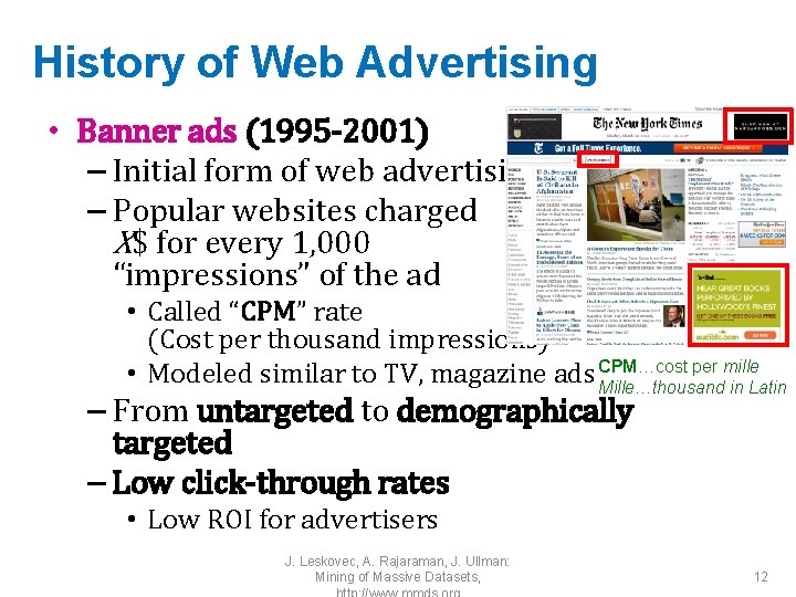
History of Web Advertising • Banner ads (1995 -2001) – Initial form of web advertising – Popular websites charged X$ for every 1, 000 “impressions” of the ad • Called “CPM” rate (Cost per thousand impressions) per mille • Modeled similar to TV, magazine ads CPM…cost Mille…thousand in Latin – From untargeted to demographically targeted – Low click-through rates • Low ROI for advertisers J. Leskovec, A. Rajaraman, J. Ullman: Mining of Massive Datasets, 12

Performance-based Advertising • Introduced by Overture around 2000 – Advertisers bid on search keywords – When someone searches for that keyword, the highest bidder’s ad is shown – Advertiser is charged only if the ad is clicked on • Similar model adopted by Google with some changes around 2002 – Called Adwords J. Leskovec, A. Rajaraman, J. Ullman: Mining of Massive Datasets, 13

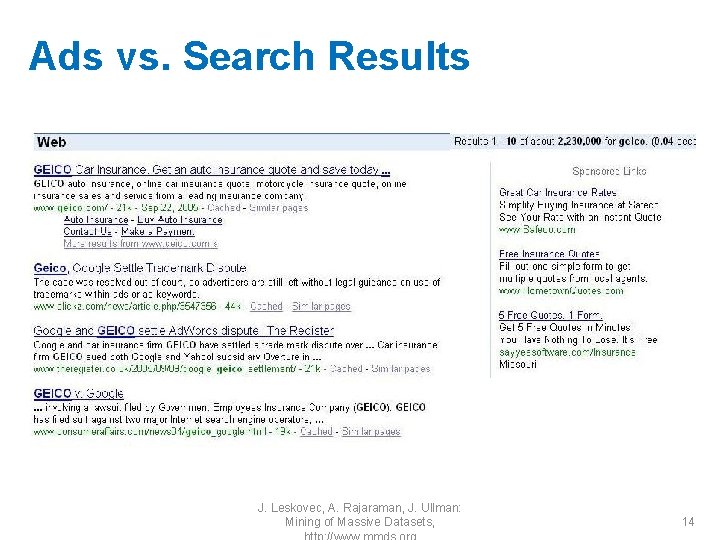
Ads vs. Search Results J. Leskovec, A. Rajaraman, J. Ullman: Mining of Massive Datasets, 14

Web 2. 0 • Performance-based advertising works! – Multi-billion-dollar industry • Interesting problem: What ads to show for a given query? – (Today’s lecture) • If I am an advertiser, which search terms should I bid on and how much should I bid? – (Not focus of today’s lecture) J. Leskovec, A. Rajaraman, J. Ullman: Mining of Massive Datasets, 15

Adwords Problem • Given: – 1. A set of bids by advertisers for search queries – 2. A click-through rate for each advertiser-query pair – 3. A budget for each advertiser (say for 1 month) – 4. A limit on the number of ads to be displayed with each search query • Respond to each search query with a set of advertisers such that: – 1. The size of the set is no larger than the limit on the number of ads per query – 2. Each advertiser has bid on the search query – 3. Each advertiser has enough budget left to pay A. Rajaraman, J. Ullman: for the ad if it J. is. Leskovec, clicked upon Mining of Massive Datasets, 16

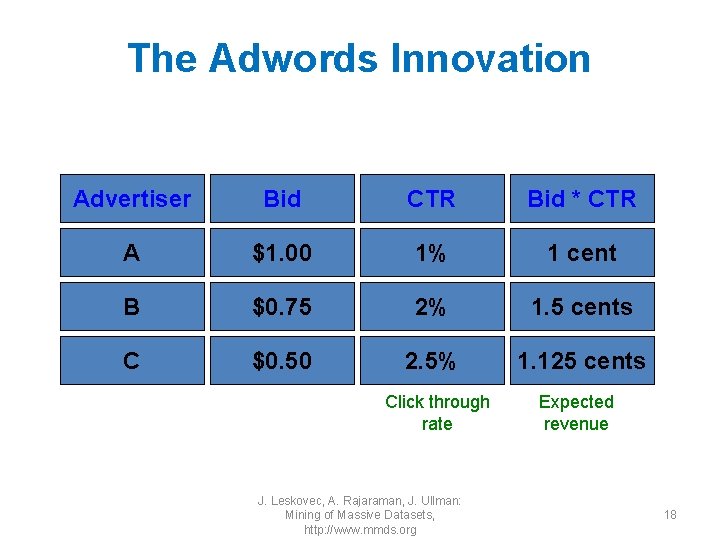
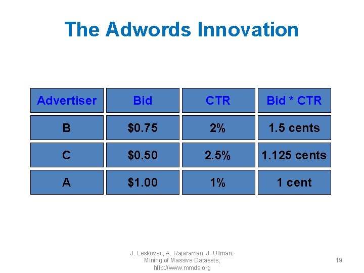
Adwords Problem • A stream of queries arrives at the search engine: q 1, q 2, … • Several advertisers bid on each query • When query qi arrives, search engine must pick a subset of advertisers whose ads are shown • Goal: Maximize search engine’s revenues – Simple solution: Instead of raw bids, use the “expected revenue per click” (i. e. , Bid*CTR) • Clearly we need an online algorithm! J. Leskovec, A. Rajaraman, J. Ullman: Mining of Massive Datasets, 17

The Adwords Innovation Advertiser Bid CTR Bid * CTR A $1. 00 1% 1 cent B $0. 75 2% 1. 5 cents C $0. 50 2. 5% 1. 125 cents Click through rate J. Leskovec, A. Rajaraman, J. Ullman: Mining of Massive Datasets, http: //www. mmds. org Expected revenue 18

The Adwords Innovation Advertiser Bid CTR Bid * CTR B $0. 75 2% 1. 5 cents C $0. 50 2. 5% 1. 125 cents A $1. 00 1% 1 cent J. Leskovec, A. Rajaraman, J. Ullman: Mining of Massive Datasets, http: //www. mmds. org 19

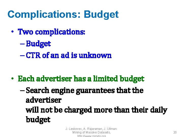
Complications: Budget • Two complications: – Budget – CTR of an ad is unknown • Each advertiser has a limited budget – Search engine guarantees that the advertiser will not be charged more than their daily budget J. Leskovec, A. Rajaraman, J. Ullman: Mining of Massive Datasets, 20

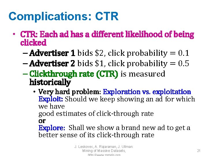
Complications: CTR • CTR: Each ad has a different likelihood of being clicked – Advertiser 1 bids $2, click probability = 0. 1 – Advertiser 2 bids $1, click probability = 0. 5 – Clickthrough rate (CTR) is measured historically • Very hard problem: Exploration vs. exploitation Exploit: Should we keep showing an ad for which we have good estimates of click-through rate or Explore: Shall we show a brand new ad to get a better sense of its click-through rate J. Leskovec, A. Rajaraman, J. Ullman: Mining of Massive Datasets, 21

BALANCE Algorithm [MSVV] • BALANCE Algorithm by Mehta, Saberi, Vazirani, and Vazirani – For each query, pick the advertiser with the largest unspent budget • Break ties arbitrarily (but in a deterministic way) J. Leskovec, A. Rajaraman, J. Ullman: Mining of Massive Datasets, 22

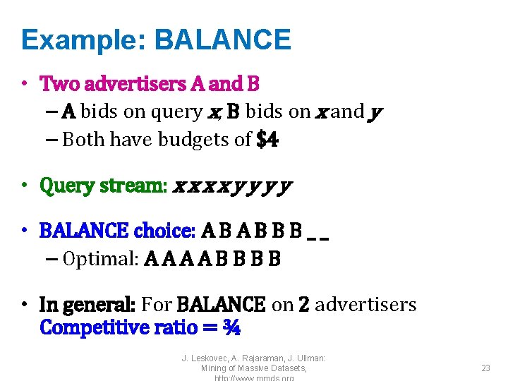
Example: BALANCE • Two advertisers A and B – A bids on query x, B bids on x and y – Both have budgets of $4 • Query stream: x x y y • BALANCE choice: A B B B _ _ – Optimal: A A B B • In general: For BALANCE on 2 advertisers Competitive ratio = ¾ J. Leskovec, A. Rajaraman, J. Ullman: Mining of Massive Datasets, 23

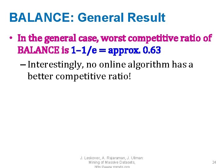
BALANCE: General Result • In the general case, worst competitive ratio of BALANCE is 1– 1/e = approx. 0. 63 – Interestingly, no online algorithm has a better competitive ratio! J. Leskovec, A. Rajaraman, J. Ullman: Mining of Massive Datasets, 24

2: Recommender Systems

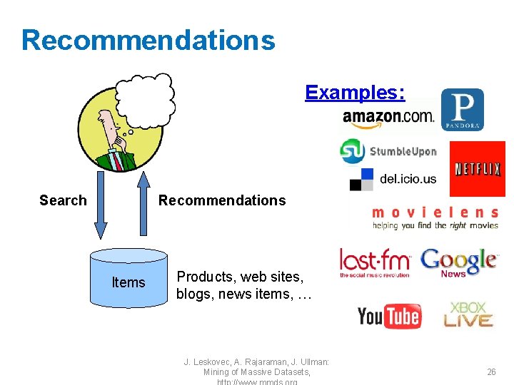
Recommendations Examples: Search Recommendations Items Products, web sites, blogs, news items, … J. Leskovec, A. Rajaraman, J. Ullman: Mining of Massive Datasets, 26

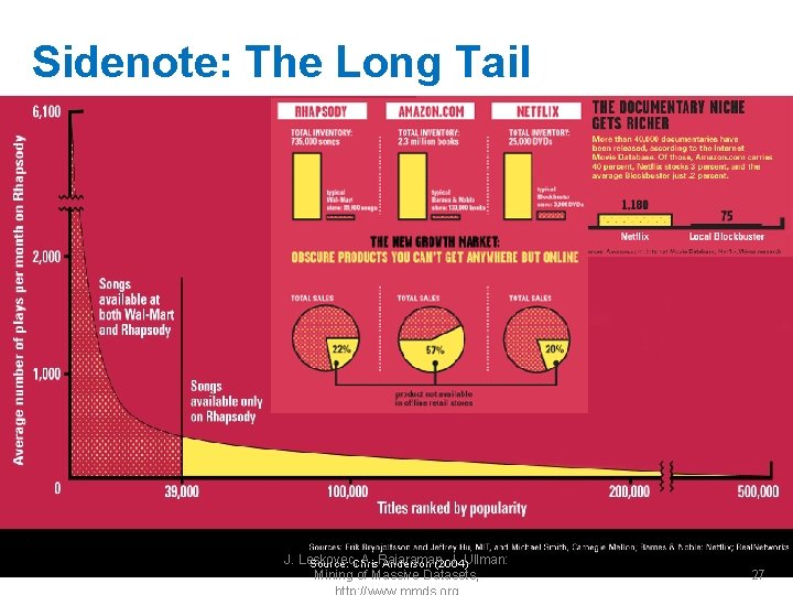
Sidenote: The Long Tail J. Leskovec, A. Rajaraman, J. Ullman: Source: Chris Anderson (2004) Mining of Massive Datasets, 27

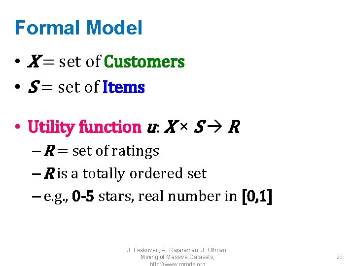
Formal Model • X = set of Customers • S = set of Items • Utility function u: X × S R – R = set of ratings – R is a totally ordered set – e. g. , 0 -5 stars, real number in [0, 1] J. Leskovec, A. Rajaraman, J. Ullman: Mining of Massive Datasets, 28

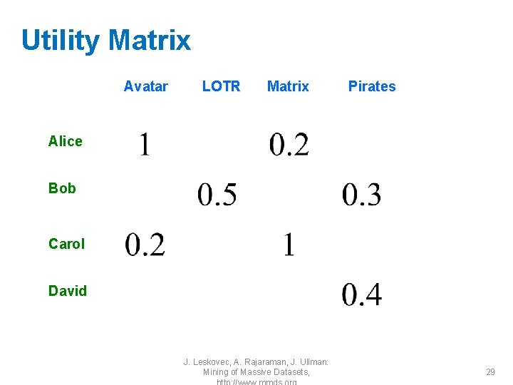
Utility Matrix Avatar LOTR Matrix Pirates Alice Bob Carol David J. Leskovec, A. Rajaraman, J. Ullman: Mining of Massive Datasets, 29

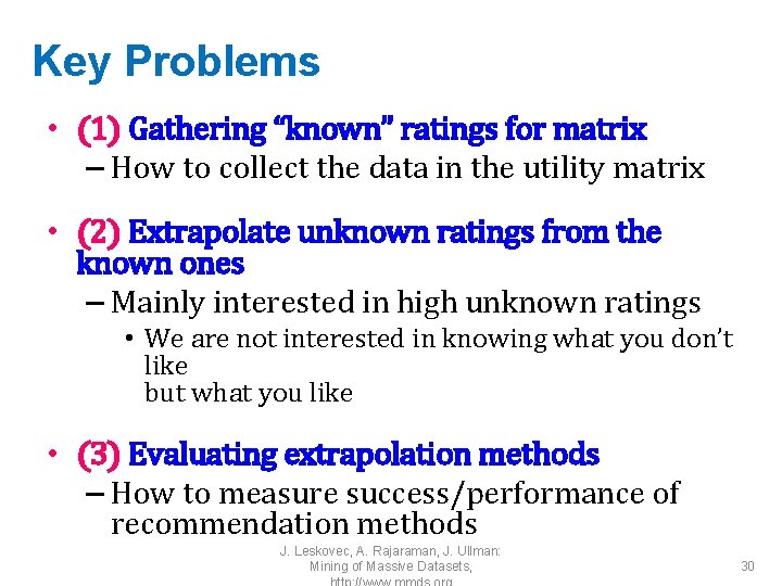
Key Problems • (1) Gathering “known” ratings for matrix – How to collect the data in the utility matrix • (2) Extrapolate unknown ratings from the known ones – Mainly interested in high unknown ratings • We are not interested in knowing what you don’t like but what you like • (3) Evaluating extrapolation methods – How to measure success/performance of recommendation methods J. Leskovec, A. Rajaraman, J. Ullman: Mining of Massive Datasets, 30

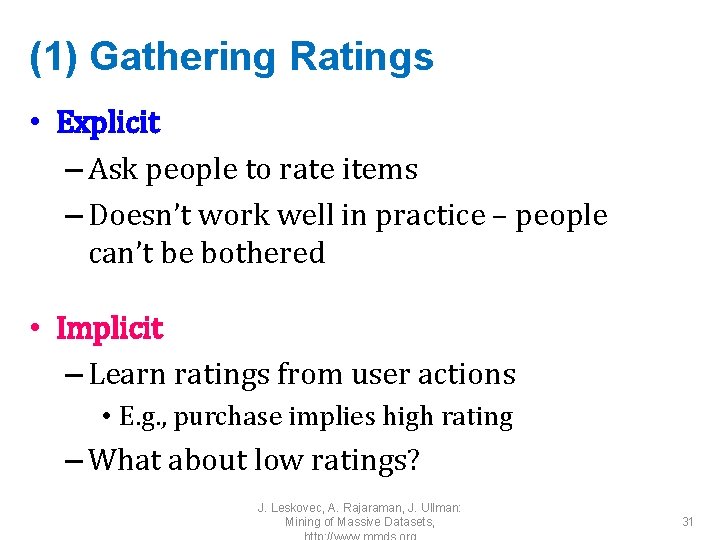
(1) Gathering Ratings • Explicit – Ask people to rate items – Doesn’t work well in practice – people can’t be bothered • Implicit – Learn ratings from user actions • E. g. , purchase implies high rating – What about low ratings? J. Leskovec, A. Rajaraman, J. Ullman: Mining of Massive Datasets, 31

(2) Extrapolating Utilities • Key problem: Utility matrix U is sparse – Most people have not rated most items – Cold start: • New items have no ratings • New users have no history • Three approaches to recommender systems: – 1) Content-based – 2) Collaborative – 3) Latent factor based J. Leskovec, A. Rajaraman, J. Ullman: Mining of Massive Datasets, 32

Content-based Recommendations • Main idea: Recommend items to customer x similar to previous items rated highly by x Example: • Movie recommendations – Recommend movies with same actor(s), director, genre, … • Websites, blogs, news – Recommend other sites with “similar” content J. Leskovec, A. Rajaraman, J. Ullman: Mining of Massive Datasets, 33

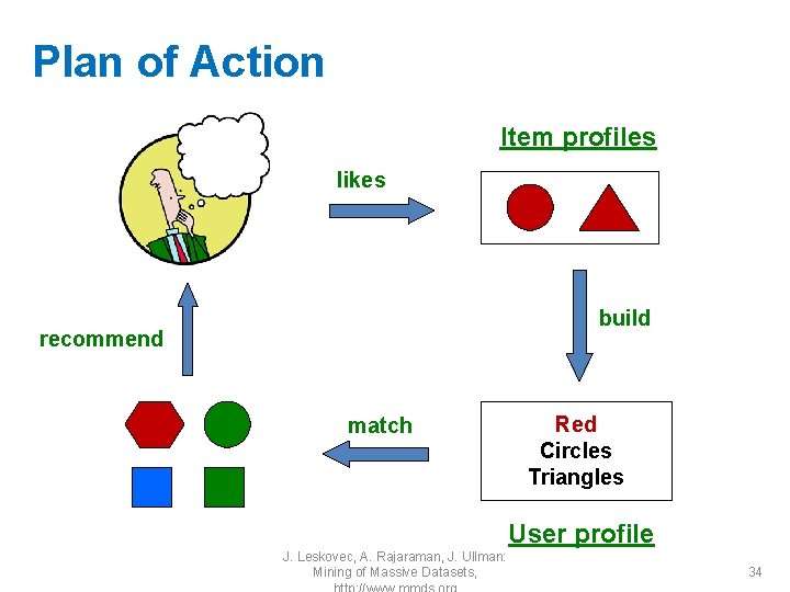
Plan of Action Item profiles likes build recommend match Red Circles Triangles User profile J. Leskovec, A. Rajaraman, J. Ullman: Mining of Massive Datasets, 34

Item Profiles • For each item, create an item profile • Profile is a set (vector) of features – Movies: author, title, actor, director, … – Text: Set of “important” words in document • How to pick important features? – Usual heuristic from text mining is TF-IDF (Term frequency * Inverse Doc Frequency) • Term … Feature • Document … Item J. Leskovec, A. Rajaraman, J. Ullman: Mining of Massive Datasets, 35

Pros: Content-based Approach • +: No need for data on other users – No cold-start or sparsity problems • +: Able to recommend to users with unique tastes • +: Able to recommend new & unpopular items – No first-rater problem • +: Able to provide explanations – Can provide explanations of recommended items by listing content-features that caused an item to be recommended J. Leskovec, A. Rajaraman, J. Ullman: Mining of Massive Datasets, 36

Cons: Content-based Approach • –: Finding the appropriate features is hard – E. g. , images, movies, music • –: Recommendations for new users – How to build a user profile? • –: Overspecialization – Never recommends items outside user’s content profile – People might have multiple interests – Unable to exploit quality judgments of other users J. Leskovec, A. Rajaraman, J. Ullman: Mining of Massive Datasets, 37

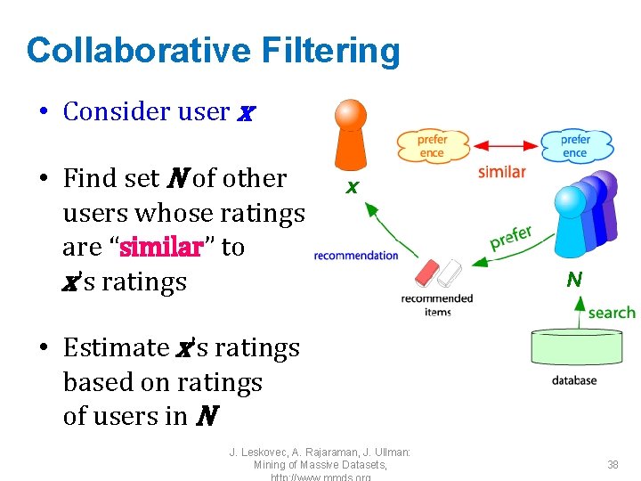
Collaborative Filtering • Consider user x • Find set N of other users whose ratings are “similar” to x’s ratings x N • Estimate x’s ratings based on ratings of users in N J. Leskovec, A. Rajaraman, J. Ullman: Mining of Massive Datasets, 38

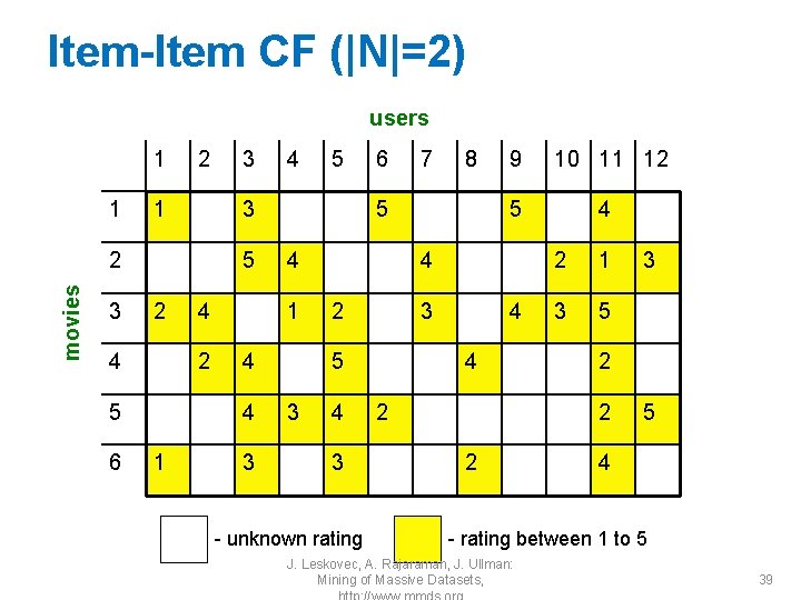
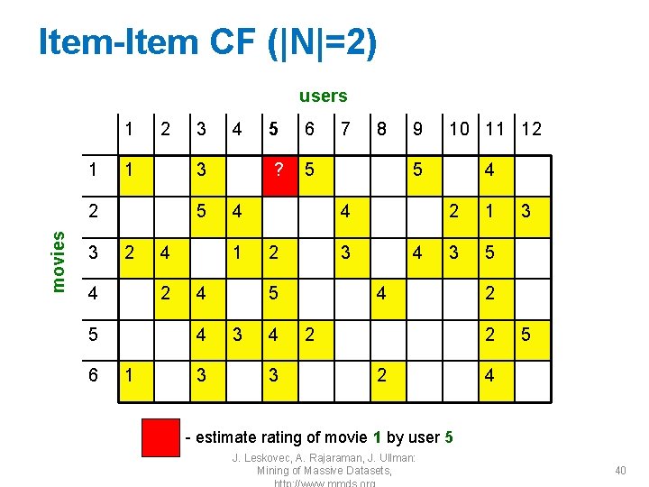
Item-Item CF (|N|=2) users 1 1 2 1 movies 5 2 4 6 4 2 5 5 4 4 3 6 7 8 5 1 4 3 2 3 3 10 11 12 5 4 4 2 3 5 3 9 4 3 - unknown rating 4 4 2 2 1 3 5 2 2 2 3 5 4 - rating between 1 to 5 J. Leskovec, A. Rajaraman, J. Ullman: Mining of Massive Datasets, 39

Item-Item CF (|N|=2) users 1 1 2 1 movies 5 2 4 6 4 2 5 4 3 5 6 ? 5 4 1 4 3 2 3 3 8 9 10 11 12 5 4 4 2 3 5 3 7 4 3 4 2 1 3 5 4 2 2 3 5 4 - estimate rating of movie 1 by user 5 J. Leskovec, A. Rajaraman, J. Ullman: Mining of Massive Datasets, 40

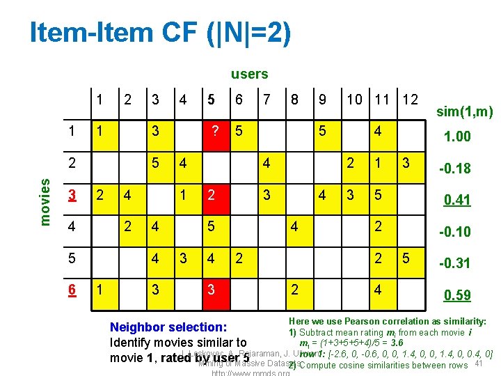
Item-Item CF (|N|=2) users 1 1 2 1 movies 5 2 4 6 4 2 5 4 3 5 6 ? 5 4 1 4 3 2 3 3 8 9 10 11 12 5 4 4 2 3 5 3 7 4 3 4 4 2 1. 00 2 1 3 5 0. 41 2 -0. 10 2 2 sim(1, m) 4 3 5 -0. 18 -0. 31 0. 59 Here we use Pearson correlation as similarity: Neighbor selection: 1) Subtract mean rating mi from each movie i m 1 = (1+3+5+5+4)/5 = 3. 6 Identify movies similar to J. Leskovec, A. Rajaraman, J. Ullman: row 1: [-2. 6, 0, -0. 6, 0, 0, 1. 4, 0, 0. 4, 0] movie 1, rated by user 5 41 Mining of Massive Datasets, 2) Compute cosine similarities between rows

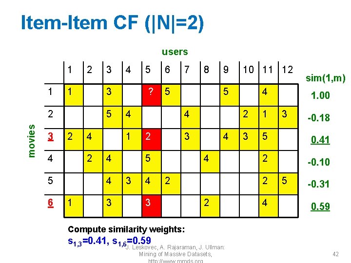
Item-Item CF (|N|=2) users 1 1 2 1 movies 5 2 4 6 4 2 5 4 3 5 6 ? 5 4 1 4 3 2 3 3 7 9 10 11 12 5 4 4 2 3 5 3 8 4 4 4 2 3 1. 00 2 1 3 5 0. 41 2 -0. 10 2 2 sim(1, m) 4 3 5 -0. 18 -0. 31 0. 59 Compute similarity weights: s 1, 3=0. 41, s 1, 6=0. 59 J. Leskovec, A. Rajaraman, J. Ullman: Mining of Massive Datasets, 42

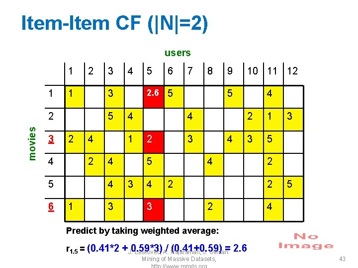
Item-Item CF (|N|=2) users 1 1 2 1 movies 5 2 4 6 4 2 5 6 4 4 3 5 7 8 2. 6 5 1 4 3 2 3 3 10 11 12 5 4 4 2 3 5 3 9 4 3 4 4 2 2 1 3 5 2 2 2 3 5 4 Predict by taking weighted average: r 1. 5 = (0. 41*2 + J. 0. 59*3) / Rajaraman, (0. 41+0. 59) = 2. 6 Leskovec, A. J. Ullman: Mining of Massive Datasets, 43

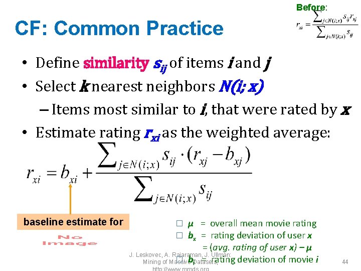
Before: CF: Common Practice • Define similarity sij of items i and j • Select k nearest neighbors N(i; x) – Items most similar to i, that were rated by x • Estimate rating rxi as the weighted average: baseline estimate for rxi μ = overall mean movie rating bx = rating deviation of user x = (avg. rating of user x) – μ J. Leskovec, A. Rajaraman, J. Ullman: � b. Datasets, Mining of Massive i = rating deviation of movie i � � 44

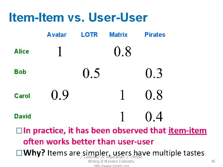
Item-Item vs. User-User Avatar LOTR Matrix Pirates Alice Bob Carol David �In practice, it has been observed that item-item often works better than user-user �Why? Items are simpler, users have multiple tastes J. Leskovec, A. Rajaraman, J. Ullman: Mining of Massive Datasets, 45

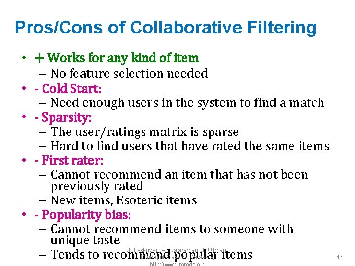
Pros/Cons of Collaborative Filtering • + Works for any kind of item – No feature selection needed • - Cold Start: – Need enough users in the system to find a match • - Sparsity: – The user/ratings matrix is sparse – Hard to find users that have rated the same items • - First rater: – Cannot recommend an item that has not been previously rated – New items, Esoteric items • - Popularity bias: – Cannot recommend items to someone with unique taste J. Leskovec, A. Rajaraman, J. Ullman: – Tends to recommend popular Mining of Massive Datasets, items 46

Hybrid Methods • Implement two or more different recommenders and combine predictions – Perhaps using a linear model • Add content-based methods to collaborative filtering – Item profiles for new item problem – Demographics to deal with new user problem J. Leskovec, A. Rajaraman, J. Ullman: Mining of Massive Datasets, 47

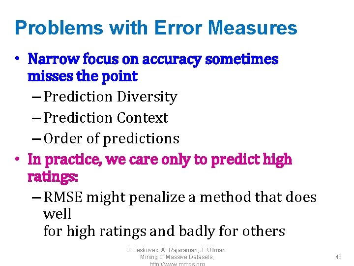
Problems with Error Measures • Narrow focus on accuracy sometimes misses the point – Prediction Diversity – Prediction Context – Order of predictions • In practice, we care only to predict high ratings: – RMSE might penalize a method that does well for high ratings and badly for others J. Leskovec, A. Rajaraman, J. Ullman: Mining of Massive Datasets, 48

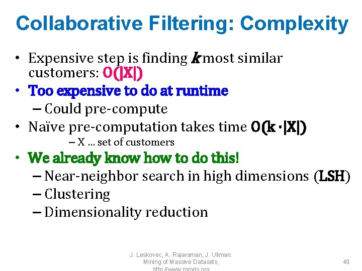
Collaborative Filtering: Complexity • Expensive step is finding k most similar customers: O(|X|) • Too expensive to do at runtime – Could pre-compute • Naïve pre-computation takes time O(k ·|X|) – X … set of customers • We already know how to do this! – Near-neighbor search in high dimensions (LSH) – Clustering – Dimensionality reduction J. Leskovec, A. Rajaraman, J. Ullman: Mining of Massive Datasets, 49

Tip: Add Data • Leverage all the data – Don’t try to reduce data size in an effort to make fancy algorithms work – Simple methods on large data do best • Add more data – e. g. , add IMDB data on genres • More data beats better algorithms http: //anand. typepad. com/datawocky/2008/03/more-data-usual. html J. Leskovec, A. Rajaraman, J. Ullman: Mining of Massive Datasets, 50

The Netflix Prize • J. Leskovec, A. Rajaraman, J. Ullman: Mining of Massive Datasets, 51

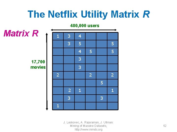
The Netflix Utility Matrix R 480, 000 users Matrix R 1 3 4 3 5 4 5 5 5 2 2 3 17, 700 movies 3 2 5 2 3 1 1 3 1 J. Leskovec, A. Rajaraman, J. Ullman: Mining of Massive Datasets, http: //www. mmds. org 52

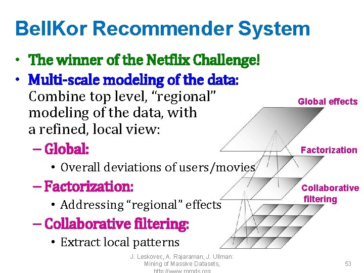
Bell. Kor Recommender System • The winner of the Netflix Challenge! • Multi-scale modeling of the data: Combine top level, “regional” modeling of the data, with a refined, local view: – Global: Global effects Factorization • Overall deviations of users/movies – Factorization: • Addressing “regional” effects Collaborative filtering – Collaborative filtering: • Extract local patterns J. Leskovec, A. Rajaraman, J. Ullman: Mining of Massive Datasets, 53

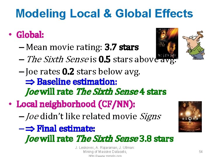
Modeling Local & Global Effects • Global: – Mean movie rating: 3. 7 stars – The Sixth Sense is 0. 5 stars above avg. – Joe rates 0. 2 stars below avg. Baseline estimation: Joe will rate The Sixth Sense 4 stars • Local neighborhood (CF/NN): – Joe didn’t like related movie Signs – Final estimate: Joe will rate The Sixth Sense 3. 8 stars J. Leskovec, A. Rajaraman, J. Ullman: Mining of Massive Datasets, 54

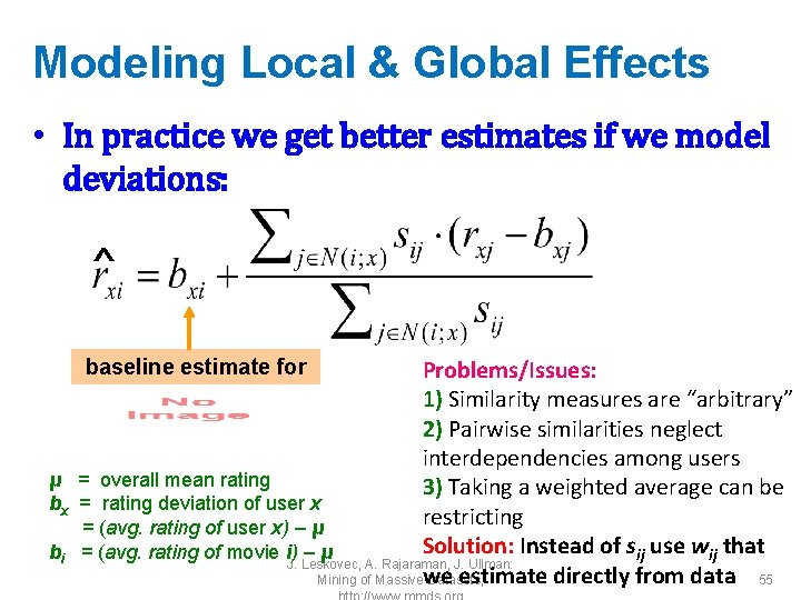
Modeling Local & Global Effects • In practice we get better estimates if we model deviations: ^ Problems/Issues: 1) Similarity measures are “arbitrary” 2) Pairwise similarities neglect interdependencies among users μ = overall mean rating 3) Taking a weighted average can be bx = rating deviation of user x restricting = (avg. rating of user x) – μ Solution: Instead of sij use wij that bi = (avg. rating of movie i) – μ J. Leskovec, A. Rajaraman, J. Ullman: estimate directly from data 55 Mining of Massivewe Datasets, baseline estimate for rxi

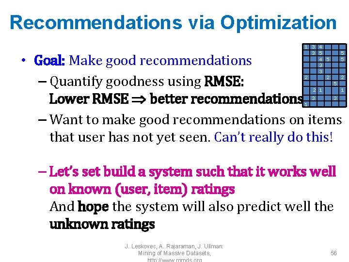
Recommendations via Optimization 1 3 4 3 5 4 5 3 3 2 2 5 5 • Goal: Make good recommendations – Quantify goodness using RMSE: Lower RMSE better recommendations – Want to make good recommendations on items that user has not yet seen. Can’t really do this! 2 1 1 3 5 3 – Let’s set build a system such that it works well on known (user, item) ratings And hope the system will also predict well the unknown ratings J. Leskovec, A. Rajaraman, J. Ullman: Mining of Massive Datasets, 56 2 1

Recommendations via Optimization • Predicted rating J. Leskovec, A. Rajaraman, J. Ullman: Mining of Massive Datasets, True rating 57

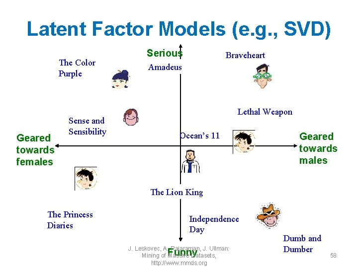
Latent Factor Models (e. g. , SVD) The Color Purple Geared towards females Sense and Sensibility Serious Braveheart Amadeus Lethal Weapon Ocean’s 11 Geared towards males The Lion King The Princess Diaries Independence Day J. Leskovec, A. Rajaraman, J. Ullman: Mining of Massive Datasets, http: //www. mmds. org Funny Dumb and Dumber 58

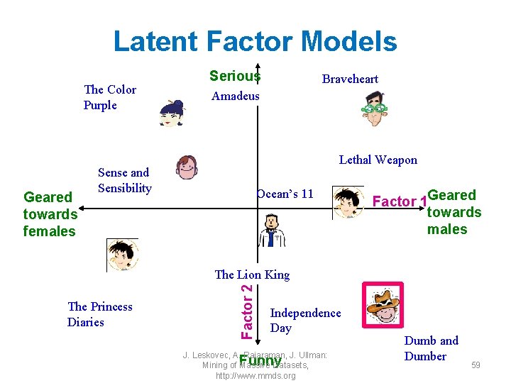
Latent Factor Models The Color Purple Geared towards females Serious Braveheart Amadeus Lethal Weapon Sense and Sensibility Ocean’s 11 Factor 1 Geared towards males The Princess Diaries Factor 2 The Lion King Independence Day J. Leskovec, A. Rajaraman, J. Ullman: Mining of Massive Datasets, http: //www. mmds. org Funny Dumb and Dumber 59

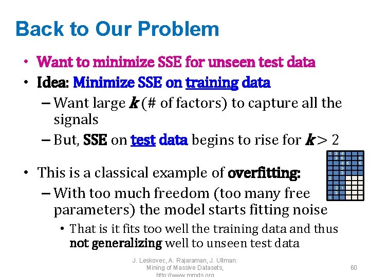
Back to Our Problem • Want to minimize SSE for unseen test data • Idea: Minimize SSE on training data – Want large k (# of factors) to capture all the signals – But, SSE on test data begins to rise for k > 2 • This is a classical example of overfitting: – With too much freedom (too many free parameters) the model starts fitting noise 1 3 4 3 5 4 5 3 3 2 ? 5 5 ? ? 2 1 3 ? ? 1 • That is it fits too well the training data and thus not generalizing well to unseen test data J. Leskovec, A. Rajaraman, J. Ullman: Mining of Massive Datasets, 60

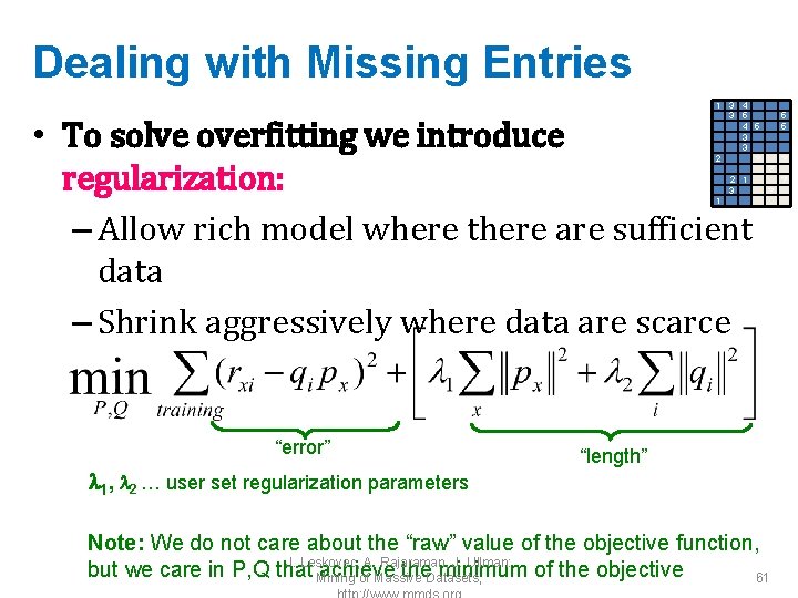
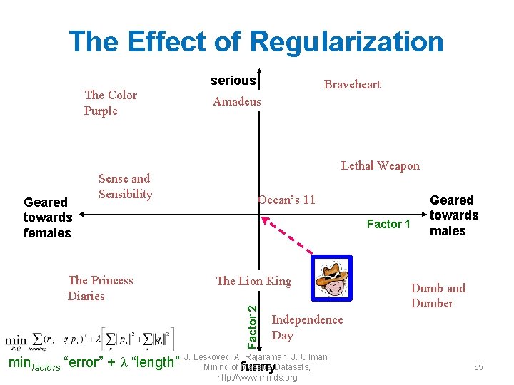
Dealing with Missing Entries 1 3 4 3 5 4 5 3 3 2 ? • To solve overfitting we introduce regularization: – Allow rich model where there are sufficient data – Shrink aggressively where data are scarce 2 1 3 5 5 ? ? 1 “error” 1, 2 … user set regularization parameters “length” Note: We do not care about the “raw” value of the objective function, J. Leskovec, A. Rajaraman, J. Ullman: but we care in P, Q that achieve the. Datasets, minimum of the objective 61 Mining of Massive

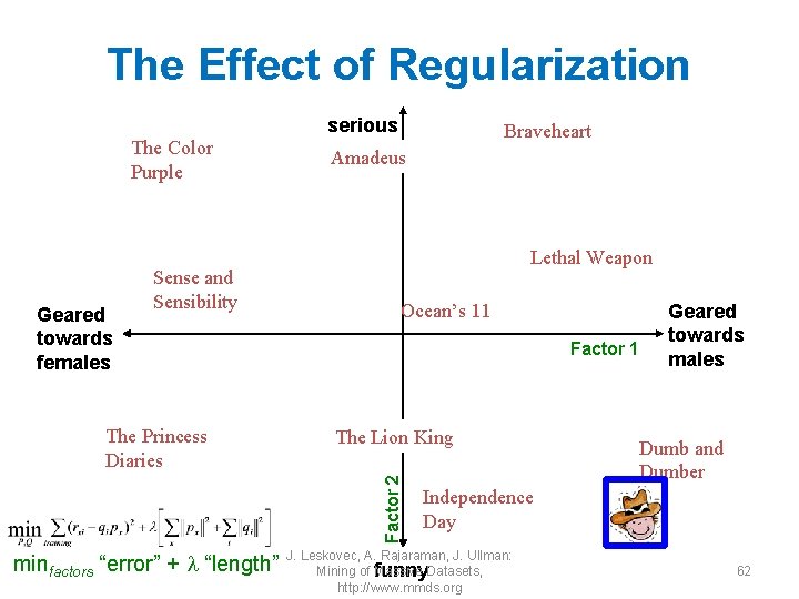
The Effect of Regularization serious The Color Purple Geared towards females Sense and Sensibility Amadeus Lethal Weapon Ocean’s 11 Factor 1 The Lion King Factor 2 The Princess Diaries Braveheart minfactors “error” + “length” Geared towards males Dumb and Dumber Independence Day J. Leskovec, A. Rajaraman, J. Ullman: Mining of Massive funny. Datasets, http: //www. mmds. org 62

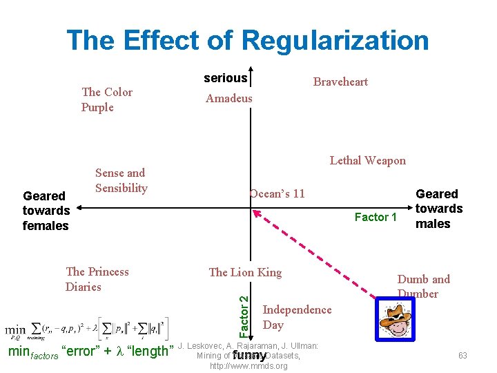
The Effect of Regularization serious The Color Purple Geared towards females Sense and Sensibility Amadeus Lethal Weapon Ocean’s 11 Factor 1 The Lion King Factor 2 The Princess Diaries Braveheart minfactors “error” + “length” Geared towards males Dumb and Dumber Independence Day J. Leskovec, A. Rajaraman, J. Ullman: Mining of Massive funny. Datasets, http: //www. mmds. org 63

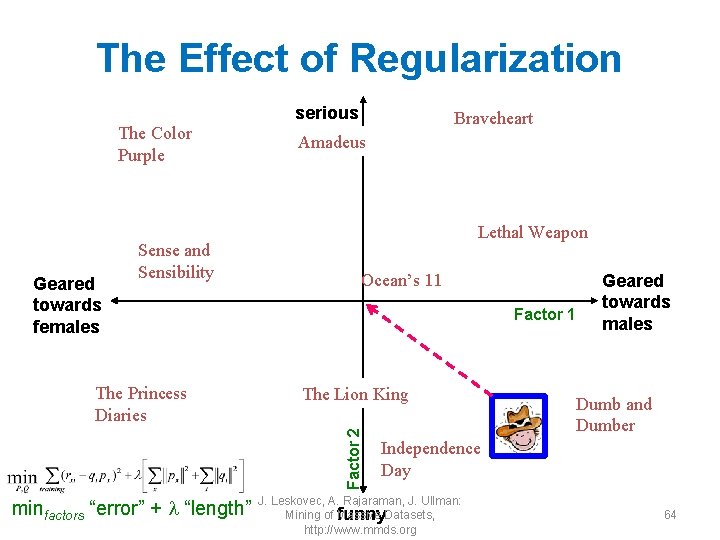
The Effect of Regularization serious The Color Purple Geared towards females Sense and Sensibility Amadeus Lethal Weapon Ocean’s 11 Factor 1 The Lion King Factor 2 The Princess Diaries Braveheart minfactors “error” + “length” Geared towards males Dumb and Dumber Independence Day J. Leskovec, A. Rajaraman, J. Ullman: Mining of Massive funny. Datasets, http: //www. mmds. org 64

The Effect of Regularization serious The Color Purple Geared towards females Sense and Sensibility Amadeus Lethal Weapon Ocean’s 11 Factor 1 The Lion King Factor 2 The Princess Diaries Braveheart minfactors “error” + “length” Geared towards males Dumb and Dumber Independence Day J. Leskovec, A. Rajaraman, J. Ullman: Mining of Massive funny. Datasets, http: //www. mmds. org 65

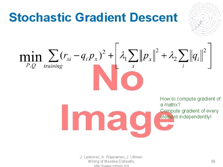
Stochastic Gradient Descent • How to compute gradient of a matrix? Compute gradient of every element independently! J. Leskovec, A. Rajaraman, J. Ullman: Mining of Massive Datasets, 66

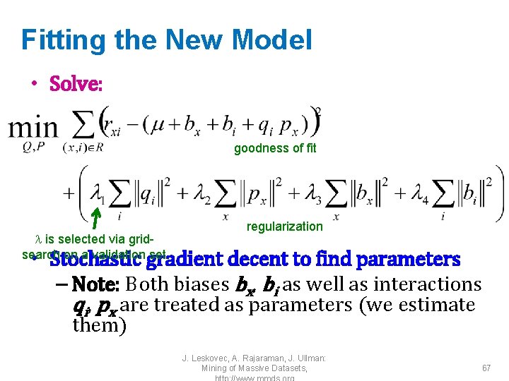
Fitting the New Model • Solve: goodness of fit is selected via gridsearch on a validation set regularization • Stochastic gradient decent to find parameters – Note: Both biases bx, bi as well as interactions qi, px are treated as parameters (we estimate them) J. Leskovec, A. Rajaraman, J. Ullman: Mining of Massive Datasets, 67

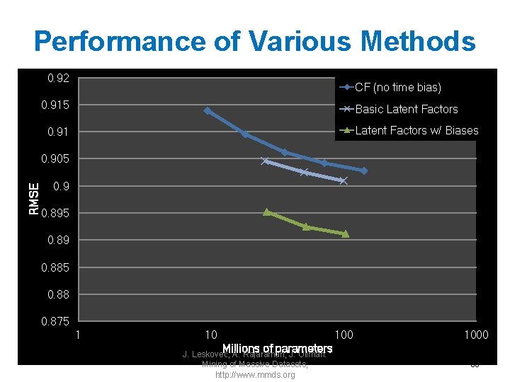
Performance of Various Methods 0. 92 CF (no time bias) 0. 915 Basic Latent Factors w/ Biases 0. 91 RMSE 0. 905 0. 9 0. 895 0. 89 0. 885 0. 88 0. 875 1 10 1000 Millions of parameters J. Leskovec, A. Rajaraman, J. Ullman: Mining of Massive Datasets, http: //www. mmds. org 68

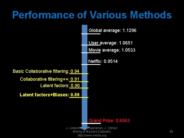
Performance of Various Methods Global average: 1. 1296 User average: 1. 0651 Movie average: 1. 0533 Netflix: 0. 9514 Basic Collaborative filtering: 0. 94 Collaborative filtering++: 0. 91 Latent factors: 0. 90 Latent factors+Biases: 0. 89 Grand Prize: 0. 8563 J. Leskovec, A. Rajaraman, J. Ullman: Mining of Massive Datasets, http: //www. mmds. org 69