Graphs Part I Shannon Quinn with thanks to

Graphs (Part I) Shannon Quinn (with thanks to William Cohen of CMU and Jure Leskovec, Anand Rajaraman, and Jeff Ullman of Stanford University)

Why I’m talking about graphs • Lots of large data is graphs – Facebook, Twitter, citation data, and other social networks – The web, the blogosphere, the semantic web, Freebase, Wikipedia, Twitter, and other information networks – Text corpora (like RCV 1), large datasets with discrete feature values, and other bipartite networks • nodes = documents or words • links connect document word or word document – Computer networks, biological networks (proteins, ecosystems, brains, …), … – Heterogeneous networks with multiple types of nodes • people, groups, documents

Properties of Graphs Descriptive Statistics • Number of connected components • Diameter • Degree distribution • … Models of Growth/Formation • Erdos-Renyi • Preferential attachment • Stochastic block models • …. Let’s look at some examples of graphs … but first, why are these statistics important?

An important question • How do you explore a dataset? – compute statistics (e. g. , feature histograms, conditional feature histograms, correlation coefficients, …) – sample and inspect • run a bunch of small-scale experiments • How do you explore a graph? – compute statistics (degree distribution, …) – sample and inspect • how do you sample?

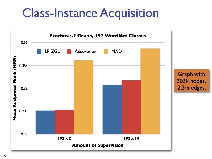
Protein-Protein Interactions Can we identify functional modules? Nodes: Proteins Edges: Physical J. Leskovec, A. Rajaraman, J. Ullman: Mining of Massive Datasets, 5

Protein-Protein Interactions Functional modules Nodes: Proteins Edges: Physical J. Leskovec, A. Rajaraman, J. Ullman: Mining of Massive Datasets, 6

Facebook Network Can we identify social communities? J. Leskovec, A. Rajaraman, J. Ullman: Mining of Massive Datasets, Nodes: Facebook Users 7

Facebook Network Social communities Summer internship High school Stanford (Basketball) Stanford (Squash) J. Leskovec, A. Rajaraman, J. Ullman: Mining of Massive Datasets, Nodes: Facebook Users 8

Blogs

Citations

Blogs

Blogs

Graphs • Set V of vertices/nodes v 1, … , set E of edges (u, v), …. – Edges might be directed and/or weighted and/or labeled • Degree of v is #edges touching v – Indegree and Outdegree for directed graphs • Path is sequence of edges (v 0, v 1), (v 1, v 2), …. • Geodesic path between u and v is shortest path connecting them – Diameter is max u, v in V {length of geodesic between u, v} – Effective diameter is 90 th percentile – Mean diameter is over connected pairs • (Connected) component is subset of nodes that are all pairwise connected via paths • Clique is subset of nodes that are all pairwise connected via edges • Triangle is a clique of size three

Graphs • Some common properties of graphs: – Distribution of node degrees – Distribution of cliques (e. g. , triangles) – Distribution of paths • Diameter (max shortest-path) • Effective diameter (90 th percentile) • Connected components – … • Some types of graphs to consider: – Real graphs (social & otherwise) – Generated graphs: • Erdos-Renyi “Bernoulli” or “Poisson” • Watts-Strogatz “small world” graphs • Barbosi-Albert “preferential attachment” • …

Erdos-Renyi graphs • Take n nodes, and connect each pair with probability p – Mean degree is z=p(n-1)

Erdos-Renyi graphs • Take n nodes, and connect each pair with probability p – Mean degree is z=p(n-1) – Mean number of neighbors distance d from v is zd – How large does d need to be so that zd >=n ? • If z>1, d = log(n)/log(z) • If z<1, you can’t do it – So: • There tend to be either many small components (z<1) or one large one (z>1) giant connected component) – Another intuition: • If there a two large connected components, then with high probability a few random edges will link them up.

Erdos-Renyi graphs • Take n nodes, and connect each pair with probability p – Mean degree is z=p(n-1) – Mean number of neighbors distance d from v is zd – How large does d need to be so that zd >=n ? • If z>1, d = log(n)/log(z) • If z<1, you can’t do it – So: • If z>1, diameters tend to be small (relative to n)

Sociometry, Vol. 32, No. 4. (Dec. , 1969), pp. 425 -443. 64 of 296 chains succeed, avg chain length is 6. 2

Illustrations of the Small World • Millgram’s experiment • Erdős numbers – http: //www. ams. org/mathscinet/searchauthors. html • Bacon numbers – http: //oracleofbacon. org/ • Linked. In – http: //www. linkedin. com/ – Privacy issues: the whole network is not visible to all

Erdos-Renyi graphs • Take n nodes, and connect each pair with probability p – Mean degree is z=p(n-1) This is usually not a good model of degree distribution in natural networks

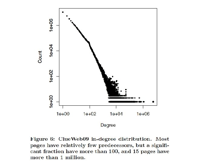
Degree distribution • Plot cumulative degree – X axis is degree – Y axis is #nodes that have degree at least k • Typically use a log-log scale – Straight lines are a power law; normal curve dives to zero at some point – Left: trust network in epinions web site from Richardson & Domingos

Degree distribution • Plot cumulative degree – X axis is degree – Y axis is #nodes that have degree at least k • Typically use a log-log scale – Straight lines are a power law; normal curve dives to zero at some point • This defines a “scale” for the network – Left: trust network in epinions web site from Richardson & Domingos

Graphs • Some common properties of graphs: – Distribution of node degrees – Distribution of cliques (e. g. , triangles) – Distribution of paths • Diameter (max shortest-path) • Effective diameter (90 th percentile) • Connected components – … • Some types of graphs to consider: – Real graphs (social & otherwise) – Generated graphs: • Erdos-Renyi “Bernoulli” or “Poisson” • Watts-Strogatz “small world” graphs • Barbosi-Albert “preferential attachment” • …

Graphs • Some common properties of graphs: – Distribution of node degrees: often scale-free – Distribution of cliques (e. g. , triangles) – Distribution of paths • Diameter (max shortestpath) • Effective diameter (90 th percentile) often small • Connected components usually one giant CC – … • Some types of graphs to consider: – Real graphs (social & otherwise) – Generated graphs: • Erdos-Renyi “Bernoulli” or “Poisson” • Watts-Strogatz “small world” graphs • Barbosi-Albert “preferential attachment” generates scale-free graphs • …

Barabasi-Albert Networks • Science 286 (1999) • Start from a small number of node, add a new node with m links • Preferential Attachment • Probability of these links to connect to existing nodes is proportional to the node’s degree • ‘Rich gets richer’ • This creates ‘hubs’: few nodes with very large degrees

Random graph (Erdos Renyi) Preferential attachment (Barabasi-Albert)

Graphs • Some common properties of graphs: – Distribution of node degrees: often scale-free – Distribution of cliques (e. g. , triangles) – Distribution of paths • Diameter (max shortestpath) • Effective diameter (90 th percentile) often small • Connected components usually one giant CC – … • Some types of graphs to consider: – Real graphs (social & otherwise) – Generated graphs: • Erdos-Renyi “Bernoulli” or “Poisson” • Watts-Strogatz “small world” graphs • Barbosi-Albert “preferential attachment” generates scale-free graphs • …

Homophily • One definition: excess edges between similar nodes – E. g. , assume nodes are male and female and Pr(male)=p, Pr(female)=q. – Is Pr(gender(u)≠ gender(v) | edge (u, v)) >= 2 pq? • Another def’n: excess edges between common neighbors of v

Homophily • Another def’n: excess edges between common neighbors of v

Homophily • In a random Erdos-Renyi graph: In natural graphs two of your mutual friends might well be friends: • Like you they are both in the same class (club, field of CS, …) • You introduced them

Watts-Strogatz model • Start with a ring • Connect each node to k nearest neighbors • homophily • Add some random shortcuts from one point to another • small diameter • Degree distribution not scale-free • Generalizes to d dimensions

An important question • How do you explore a dataset? – compute statistics (e. g. , feature histograms, conditional feature histograms, correlation coefficients, …) – sample and inspect • run a bunch of small-scale experiments • How do you explore a graph? – compute statistics (degree distribution, …) – sample and inspect • how do you sample?

KDD 2006

Brief summary • Define goals of sampling: – “scale-down” – find G’<G with similar statistics – “back in time”: for a growing G, find G’<G that is similar (statistically) to an earlier version of G • Experiment on real graphs with plausible sampling methods, such as – RN – random nodes, sampled uniformly –… • See how well they perform

Brief summary • Experiment on real graphs with plausible sampling methods, such as – RN – random nodes, sampled uniformly • RPN – random nodes, sampled by Page. Rank • RDP – random nodes sampled by in-degree – RE – random edges – RJ – run Page. Rank’s “random surfer” for n steps – RW – run RWR’s “random surfer” for n steps – FF – repeatedly pick r(i) neighbors of i to “burn”, and then recursively sample from them

10% sample – pooled on five datasets

d-statistic measures agreement between distributions • D=max{|F(x)-F’(x)|} where F, F’ are cdf’s • max over nine different statistics

Parallel Graph Computation • Distributed computation and/or multicore parallelism – Sometimes confusing. We will talk mostly about distributed computation. • Are classic graph algorithms parallelizable? What about distributed? – Depth-first search? – Breadth-first search? – Priority-queue based traversals (Djikstra’s, Prim’s algorithms)

Map. Reduce for Graphs • Graph computation almost always iterative • Map. Reduce ends up shipping the whole graph on each iteration over the network (map>reduce->map->reduce->. . . ) – Mappers and reducers are stateless

Iterative Computation is Difficult • System is not optimized for iteration: Iterations Data CPU 1 Data CPU 2 CPU 3 Data Data CPU 2 CPU 3 Disk Penalty CPU 3 Data Startup Penalty Data CPU 1 Disk Penalty Data Disk Penalty Startup Penalty CPU 2 Data Startup Penalty Data Data Data

Map. Reduce and Partitioning • Map-Reduce splits the keys randomly between mappers/reducers • But on natural graphs, high-degree vertices (keys) may have million-times more edges than the average Extremely uneven distribution Time of iteration = time of slowest job.

Curse of the Slow Job Iterations Data CPU 1 Data Data CPU 2 Data Data CPU 3 Data Data Barrier Data http: //www. www 2011 india. com/proceedings/p 607. p

Map-Reduce is Bulk-Synchronous Parallel • Bulk-Synchronous Parallel = BSP (Valiant, 80 s) – Each iteration sees only the values of previous iteration. – In linear systems literature: Jacobi iterations • Pros: – Simple to program – Maximum parallelism – Simple fault-tolerance • Cons: – Slower convergence – Iteration time = time taken by the slowest node

Triangle Counting in Twitter Graph Total: 34. 8 Billion Triangles 40 M Users 1. 2 B Edges Hadoop Graph. Lab 1536 Machines 423 Minutes 64 Machines, 1024 Cores 1. 5 Minutes Hadoop results from [Suri & Vassilvitskii '11]

Page. Rank 5. 5 hrs Hadoop Twister Graph. Lab 1 hr 8 min 40 M Webpages, 1. 4 Billion Links (100 iterations) Hadoop results from [Kang et al. '11] Twister (in-memory Map. Reduce) [Ekanayake et al. ‘ 10]

Graph algorithms • Page. Rank implementations – in memory – streaming, node list in memory – streaming, no memory – map-reduce • A little like Naïve Bayes variants – data in memory – word counts in memory – stream-and-sort – map-reduce

Google’s Page. Rank web site xxx web site a b cdefg web site yyyy pdq. . web site a b cdefg web site yyyy Inlinks are “good” (recommendations) Inlinks from a “good” site are better than inlinks from a “bad” site but inlinks from sites with many outlinks are not as “good”. . . “Good” and “bad” are relative.

Google’s Page. Rank web site xxx • follows a random link, or web site a b cdefg web site yyyy pdq. . web site a b cdefg web site yyyy Imagine a “pagehopper” that always either • jumps to random page

Google’s Page. Rank (Brin & Page, http: //www-db. stanford. edu/~backrub/google. html) web site xxx • follows a random link, or web site a b cdefg web site yyyy pdq. . web site a b cdefg web site yyyy Imagine a “pagehopper” that always either • jumps to random page Page. Rank ranks pages by the amount of time the pagehopper spends on a page: • or, if there were many pagehoppers, Page. Rank is the expected “crowd size”

Random Walks avoids messy “dead ends”….

Random Walks: Page. Rank

Random Walks: Page. Rank

Graph = Matrix Vector = Node Weight v M A B C A _ 1 1 B 1 _ C 1 1 D E F G H I J 1 A A 3 1 B 2 _ C 3 D _ 1 1 D E 1 _ 1 E 1 1 _ F F G 1 _ H 1 1 G _ 1 1 H I 1 1 _ 1 I J 1 1 1 _ J M C B A G I H D J F E

Page. Rank in Memory • Let u = (1/N, …, 1/N) – dimension = #nodes N • Let A = adjacency matrix: [aij=1 i links to j] • Let W = [wij = aij/outdegree(i)] – wij is probability of jump from i to j • Let v 0 = (1, 1, …. , 1) – or anything else you want • Repeat until converged: – Let vt+1 = cu + (1 -c)Wvt • c is probability of jumping “anywhere randomly”

Streaming Page. Rank • Assume we can store v but not W in memory • Repeat until converged: – Let vt+1 = cu + (1 -c)Wvt • Store A as a row matrix: each line is – i ji, 1, …, ji, d [the neighbors of i] • Store v’ and v in memory: v’ starts out as cu • For each line “i ji, 1, …, ji, d “ – For each j in ji, 1, …, ji, d Everything needed for update is right • v’[j] += (1 -c)v[i]/d there in row….

Streaming Page. Rank: with some long rows • Repeat until converged: – Let vt+1 = cu + (1 -c)Wvt • Store A as a list of edges: each line is: “i d(i) j” • Store v’ and v in memory: v’ starts out as cu • For each line “i d j“ • v’[j] += (1 -c)v[i]/d We need to get the degree of i and store it locally

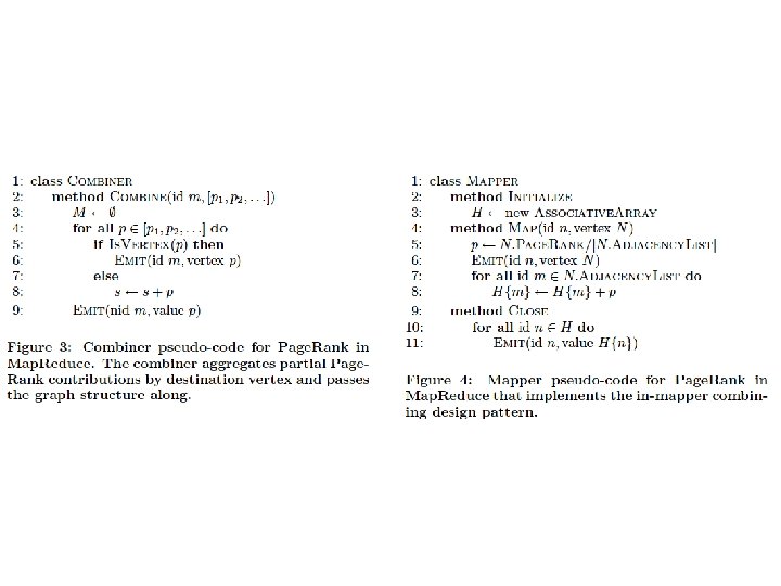
Streaming Page. Rank: preprocessing • • Original encoding is edges (i, j) Mapper replaces i, j with i, 1 Reducer is a Sum. Reducer Result is pairs (i, d(i)) • Then: join this back with edges (i, j) • For each i, j pair: – send j as a message to node i in the degree table • messages always sorted after non-messages – the reducer for the degree table sees i, d(i) first • then j 1, j 2, …. • can output the key, value pairs with key=i, value=d(i), j

Page. Rank in Map. Reduce

More on graph algorithms • Page. Rank is a one simple example of a graph algorithm – but an important one – personalized Page. Rank (aka “random walk with restart”) is an important operation in machine learning/data analysis settings • Page. Rank is typical in some ways – Trivial when graph fits in memory – Easy when node weights fit in memory – More complex to do with constant memory – A major expense is scanning through the graph many times • … same as with SGD/Logistic regression • disk-based streaming is much more expensive than memory-based approaches • Locality of access is very important! • gains if you can pre-cluster the graph even approximately • avoid sending messages across the network – keep them local

Machine Learning in Graphs - 2010

Some ideas • Combiners are helpful – Store outgoing increment. VBy messages and aggregate them – This is great for high indegree pages • Hadoop’s combiners are suboptimal – Messages get emitted before being combined – Hadoop makes weak guarantees about combiner usage

This slide again!

Some ideas • Most hyperlinks are within a domain – If we keep domains on the same machine this will mean more messages are local – To do this, build a custom partitioner that knows about the domain of each node. Id and keeps nodes on the same domain together – Assign node id’s so that nodes in the same domain are together – partition node ids by range – Change Hadoop’s Partitioner for this

Some ideas • Repeatedly shuffling the graph is expensive – We should separate the messages about the graph structure (fixed over time) from messages about page. Rank weights (variable) – compute and distribute the edges once – read them in incrementally in the reducer • not easy to do in Hadoop! – call this the “Schimmy” pattern

Schimmy Relies on fact that keys are sorted, and sorts the graph input the same way…. .

Schimmy

Results

More details at… • Overlapping Community Detection at Scale: A Nonnegative Matrix Factorization Approach by J. Yang, J. Leskovec. ACM International Conference on Web Search and Data Mining (WSDM), 2013. • Detecting Cohesive and 2 -mode Communities in Directed and Undirected Networks by J. Yang, J. Mc. Auley, J. Leskovec. ACM International Conference on Web Search and Data Mining (WSDM), 2014. • Community Detection in Networks with Node Attributes by J. Yang, J. Mc. Auley, J. Leskovec. IEEE International Conference On Data Mining (ICDM), 2013. J. Leskovec, A. Rajaraman, J. Ullman: Mining of Massive Datasets, 71

Semi-Supervised Learning With Graphs Shannon Quinn (with thanks to William Cohen at CMU)

Semi-supervised learning • A pool of labeled examples L • A (usually larger) pool of unlabeled examples U • Can you improve accuracy somehow using U?

Semi-Supervised Bootstrapped Learning/Self-training Extract cities: Paris Pittsburgh Seattle Cupertino San Francisco Austin denial mayor of arg 1 live in arg 1 anxiety selfishness Berlin arg 1 is home of traits such as arg 1

Semi-Supervised Bootstrapped Learning via Label Propagation mayor of arg 1 Paris Pittsburgh arg 1 is home of San Francisco Austin anxiety live in arg 1 traits such as arg 1 denial Seattle selfishness

Semi-Supervised Bootstrapped Learning via Label Propagation mayor of arg 1 Paris Pittsburgh arg 1 is home of San Francisco Austin traits such as arg 1 live in arg 1 denial Seattle Nodes “near” seeds Information from other categories tells youanxiety “how far” (when to stop propagating) arrogance selfishness Nodes “far from” seeds

ASONAM-2010 (Advances in Social Networks Analysis and Mining)

Network Datasets with Known Classes • UBMCBlog • AGBlog • MSPBlog • Cora • Citeseer

RWR - fixpoint of: Seed selection 1. order by Page. Rank, degree, or randomly 2. go down list until you have at least k examples/class

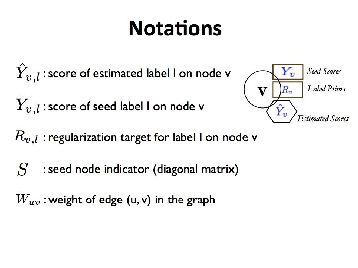
Co. EM/HF/wv. RN • One definition [Mac. Skassy & Provost, JMLR 2007]: …

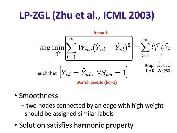
Co. EM/HF/wv. RN • Another definition in [X. Zhu, Z. Ghahramani, and J. Lafferty, ICML 2003] – A harmonic field – the score of each node in the graph is the harmonic, or linearly weighted, average of its neighbors’ scores (harmonic field, HF)

Co. EM/HF/wv. RN • Another justification of the same algorithm…. • … start with co -training with a naïve Bayes learner

How to do this minimization? First, differentiate to find min is at Jacobi method: • To solve Ax=b for x • Iterate: • … or: