Realdata WRF Setup and run ATM 419563 Spring

Real-data WRF: Setup and run ATM 419/563 Spring 2020 Fovell 1 © Copyright 2020 Robert Fovell, Univ. at Albany, SUNY, rfovell@albany. edu

References • WRFV 4 users guide (PDF available) – http: //www 2. mmm. ucar. edu/wrf/users/docs/user_guide_ v 4/contents. html • Technical description of WRFV 3 (PDF) – http: //www 2. mmm. ucar. edu/wrf/users/docs/arw_v 3. pdf • Net. CDF operators (NCO) home page • IDV home page 2

Terms & facts • Parent model = gridded data used for initialization and boundary conditions – GFS/FNL, NAM, RAP/HRRR, reanalyses (NARR, CFSR, NNRP, ERA-interim, ERA-5 etc. ), other WRF runs • WPS = WRF Preprocessing System (consisting of geogrid, ungrib, and metgrid programs) • WRF simulations are almost always initialized with parent model datasets on isobaric levels in GRIB 1/2 format, or WRF outputs in Net. CDF format • WRF outputs are almost always Net. CDF 3

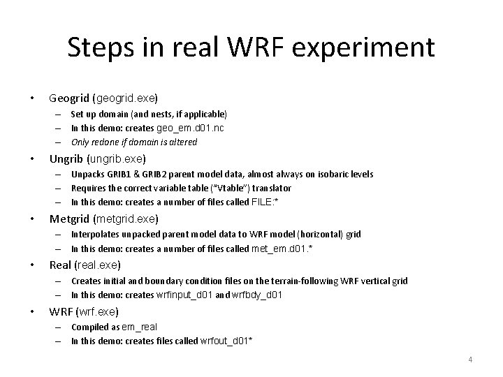
Steps in real WRF experiment • Geogrid (geogrid. exe) – Set up domain (and nests, if applicable) – In this demo: creates geo_em. d 01. nc – Only redone if domain is altered • Ungrib (ungrib. exe) – Unpacks GRIB 1 & GRIB 2 parent model data, almost always on isobaric levels – Requires the correct variable table (“Vtable”) translator – In this demo: creates a number of files called FILE: * • Metgrid (metgrid. exe) – Interpolates unpacked parent model data to WRF model (horizontal) grid – In this demo: creates a number of files called met_em. d 01. * • Real (real. exe) – Creates initial and boundary condition files on the terrain-following WRF vertical grid – In this demo: creates wrfinput_d 01 and wrfbdy_d 01 • WRF (wrf. exe) – Compiled as em_real – In this demo: creates files called wrfout_d 01* 4

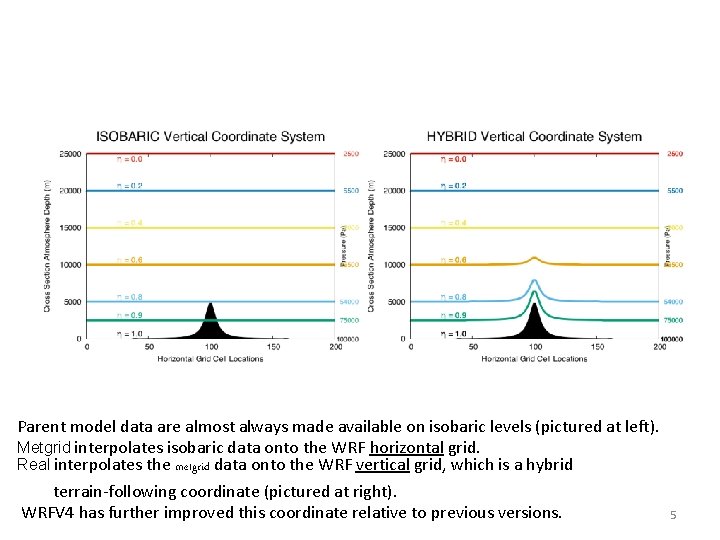
Parent model data are almost always made available on isobaric levels (pictured at left). Metgrid interpolates isobaric data onto the WRF horizontal grid. Real interpolates the metgrid data onto the WRF vertical grid, which is a hybrid terrain-following coordinate (pictured at right). WRFV 4 has further improved this coordinate relative to previous versions. 5

Case study • One 36 -km resolution, 54 x 48 point domain centered over Kansas, simulated using WRF version 4. 1. 1 • 48 h simulation, initialized from GFS at 3/13/2016 at 00 Z, with hourly outputs • Verify near-surface fields (T, Td, RH at 2 m; 10 -m wind; SLP) against ASOS stations using Model Evaluation Tools (MET) package • See provided script for implementing this case study 6

Preliminaries • WRF-ARW has been compiled as em_real • Namelists are – namelist. wps (used for geogrid. exe, ungrib. exe, metgrid. exe) – namelist. input (used for real. exe, wrf. exe) • In your lab space, create a directory called KANSAS, move into it, and copy/unpack this file – $LAB/KANSAS/SETUP. tar 7

make_all_links. sh • This file is different and not interchangeable with versions supporting idealized runs • In addition to linking to needed programs and support files for WRF real, this shell script also: – Creates directories called geogrid and metgrid, and places the default *. TBL files in them. We do not need to alter those files at this time. – Copies variable translation tables, called Vtable. *, for commonly used parent model datasets 8

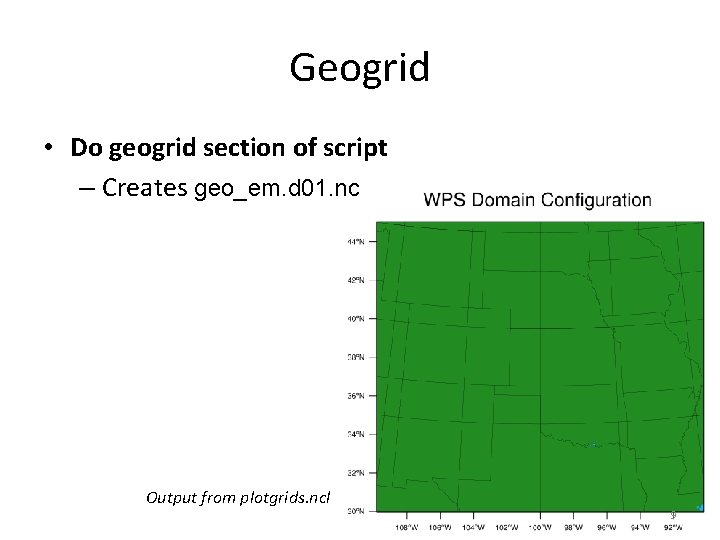
Geogrid • Do geogrid section of script – Creates geo_em. d 01. nc Output from plotgrids. ncl 9

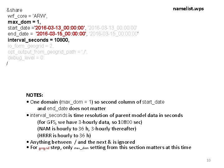
&share wrf_core = 'ARW', max_dom = 1, start_date ='2016 -03 -13_00: 00', '2016 -03 -13_00: 00' end_date = '2016 -03 -15_00: 00', '2016 -03 -15_00: 00' interval_seconds = 10800, io_form_geogrid = 2, opt_output_from_geogrid_path = '. /', debug_level = 0 / namelist. wps NOTES: • One domain (max_dom = 1) so second column of start_date and end_date does not matter • interval_seconds is time resolution of parent model data in seconds (for GFS, we have 3 -hourly data, so 10800 sec) (NAM is hourly to 36 h, 3 -hourly thereafter) (HRRR is hourly to 36 h) • Anything between / and the next & is ignored • For geogrid step, only max_dom setting from this section matters at this time 10

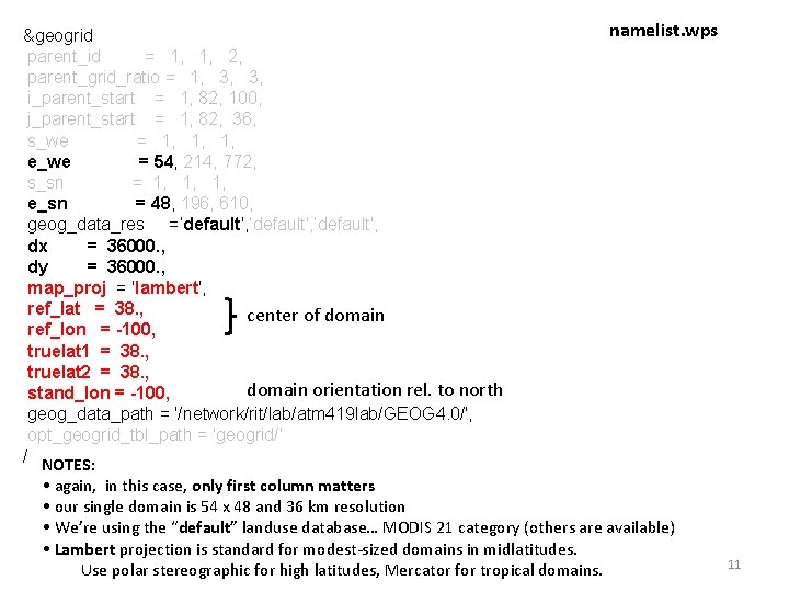
&geogrid parent_id = 1, 1, 2, parent_grid_ratio = 1, 3, 3, i_parent_start = 1, 82, 100, j_parent_start = 1, 82, 36, s_we = 1, 1, 1, e_we = 54, 214, 772, s_sn = 1, 1, 1, e_sn = 48, 196, 610, geog_data_res =’default', dx = 36000. , dy = 36000. , map_proj = 'lambert', ref_lat = 38. , center of domain ref_lon = -100, truelat 1 = 38. , truelat 2 = 38. , domain orientation rel. to north stand_lon = -100, geog_data_path = '/network/rit/lab/atm 419 lab/GEOG 4. 0/', opt_geogrid_tbl_path = 'geogrid/' / NOTES: namelist. wps • again, in this case, only first column matters • our single domain is 54 x 48 and 36 km resolution • We’re using the “default” landuse database… MODIS 21 category (others are available) • Lambert projection is standard for modest-sized domains in midlatitudes. Use polar stereographic for high latitudes, Mercator for tropical domains. 11

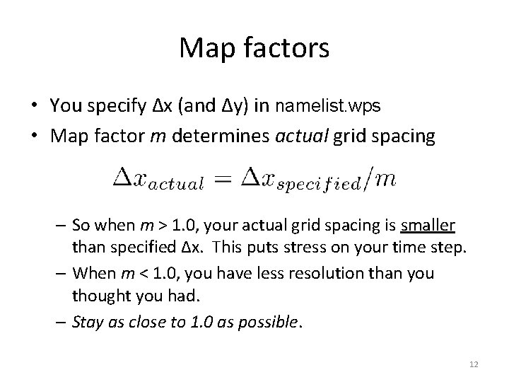
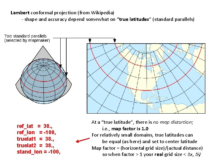
Map factors • You specify ∆x (and ∆y) in namelist. wps • Map factor m determines actual grid spacing – So when m > 1. 0, your actual grid spacing is smaller than specified ∆x. This puts stress on your time step. – When m < 1. 0, you have less resolution than you thought you had. – Stay as close to 1. 0 as possible. 12

Lambert conformal projection (from Wikipedia) - shape and accuracy depend somewhat on “true latitudes” (standard parallels) ref_lat = 38. , ref_lon = -100, truelat 1 = 38. , truelat 2 = 38. , stand_lon = -100, At a “true latitude”, there is no map distortion; i. e. , map factor is 1. 0 For relatively small domains, true latitudes can be equal (as here) and set to center latitude Map factor = (horizontal grid size)/(actual distance) 13 so when factor > 1 your real grid size < ∆x, ∆y

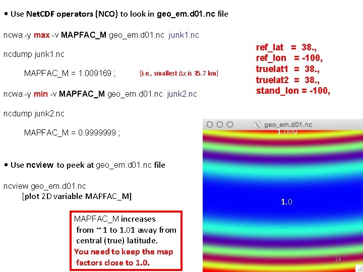
• Use Net. CDF operators (NCO) to look in geo_em. d 01. nc file ncwa -y max -v MAPFAC_M geo_em. d 01. nc junk 1. nc ncdump junk 1. nc MAPFAC_M = 1. 009169 ; [i. e. , smallest ∆x is 35. 7 km] ncwa -y min -v MAPFAC_M geo_em. d 01. nc junk 2. nc ref_lat = 38. , ref_lon = -100, truelat 1 = 38. , truelat 2 = 38. , stand_lon = -100, ncdump junk 2. nc MAPFAC_M = 0. 9999999 ; 1. 009 • Use ncview to peek at geo_em. d 01. nc file ncview geo_em. d 01. nc [plot 2 D variable MAPFAC_M] 1. 0 MAPFAC_M increases from ~ 1 to 1. 01 away from central (true) latitude. You need to keep the map factors close to 1. 0. 14

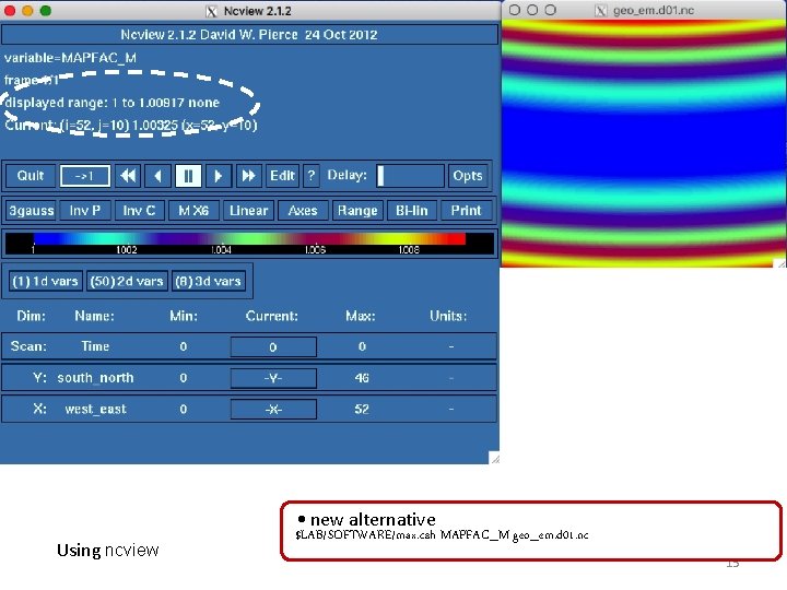
• new alternative Using ncview $LAB/SOFTWARE/max. csh MAPFAC_M geo_em. d 01. nc 15

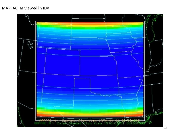
MAPFAC_M viewed in IDV 16

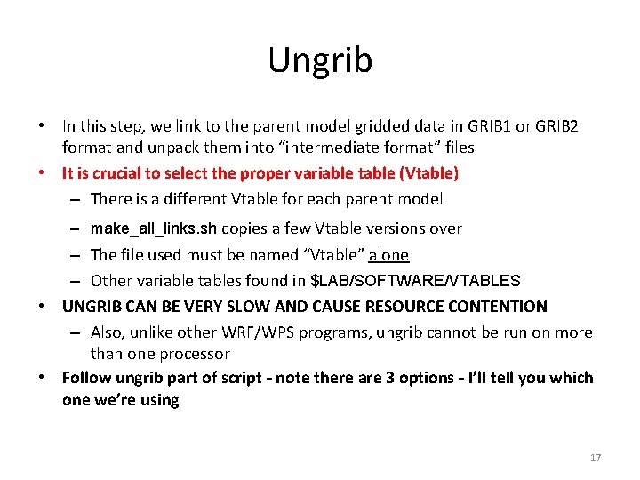
Ungrib • In this step, we link to the parent model gridded data in GRIB 1 or GRIB 2 format and unpack them into “intermediate format” files • It is crucial to select the proper variable table (Vtable) – There is a different Vtable for each parent model – make_all_links. sh copies a few Vtable versions over – The file used must be named “Vtable” alone – Other variable tables found in $LAB/SOFTWARE/VTABLES • UNGRIB CAN BE VERY SLOW AND CAUSE RESOURCE CONTENTION – Also, unlike other WRF/WPS programs, ungrib cannot be run on more than one processor • Follow ungrib part of script – note there are 3 options – I’ll tell you which one we’re using 17

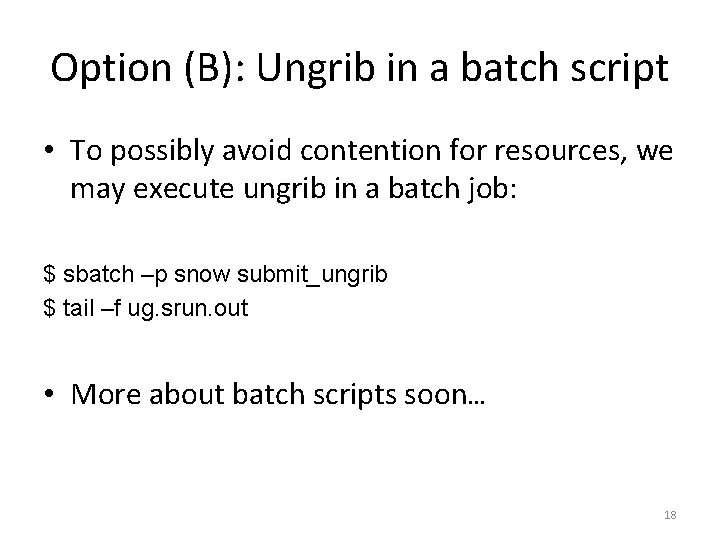
Option (B): Ungrib in a batch script • To possibly avoid contention for resources, we may execute ungrib in a batch job: $ sbatch –p snow submit_ungrib $ tail –f ug. srun. out • More about batch scripts soon… 18

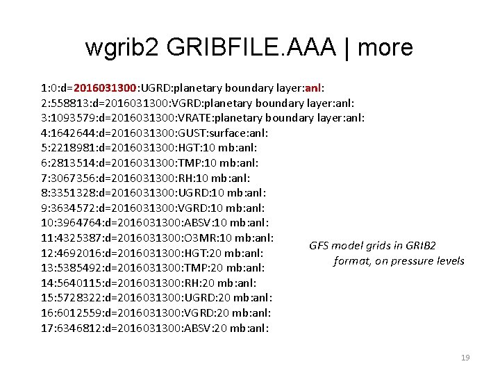
wgrib 2 GRIBFILE. AAA | more 1: 0: d=2016031300: UGRD: planetary boundary layer: anl: 2: 558813: d=2016031300: VGRD: planetary boundary layer: anl: 3: 1093579: d=2016031300: VRATE: planetary boundary layer: anl: 4: 1642644: d=2016031300: GUST: surface: anl: 5: 2218981: d=2016031300: HGT: 10 mb: anl: 6: 2813514: d=2016031300: TMP: 10 mb: anl: 7: 3067356: d=2016031300: RH: 10 mb: anl: 8: 3351328: d=2016031300: UGRD: 10 mb: anl: 9: 3634572: d=2016031300: VGRD: 10 mb: anl: 10: 3964764: d=2016031300: ABSV: 10 mb: anl: 11: 4325387: d=2016031300: O 3 MR: 10 mb: anl: GFS model grids in GRIB 2 12: 4692016: d=2016031300: HGT: 20 mb: anl: format, on pressure levels 13: 5385492: d=2016031300: TMP: 20 mb: anl: 14: 5640115: d=2016031300: RH: 20 mb: anl: 15: 5728322: d=2016031300: UGRD: 20 mb: anl: 16: 6012559: d=2016031300: VGRD: 20 mb: anl: 17: 6346812: d=2016031300: ABSV: 20 mb: anl: 19

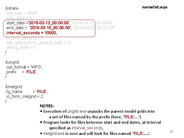
&share wrf_core = 'ARW', max_dom = 1, start_date ='2016 -03 -13_00: 00', '2016 -03 -13_00: 00' end_date = '2016 -03 -15_00: 00', '2016 -03 -15_00: 00' interval_seconds = 10800, io_form_geogrid = 2, opt_output_from_geogrid_path = '. /', debug_level = 0 / namelist. wps &ungrib out_format = 'WPS', prefix = 'FILE', / &metgrid fg_name = 'FILE', io_form_metgrid = 2, / NOTES: • Execution of ungrib. exe unpacks the parent model grids into a set of files named by the prefix (here, ‘FILE: …’) • Program looks for files between start and end dates, at interval specified as interval_seconds. • metgrid. exe is next and will look for files named ‘FILE: …’. 20

Plotting intermediate format files created by ungrib. exe [OPTIONAL] ncl plotfmt. ncl 'filename="FILE: 2016 -03 -13_00"' It is possible to plot parent model data directly from the GRIB files with Gr. ADS and Python tools 21

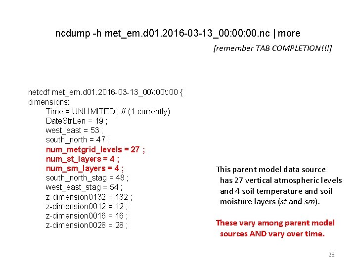
Metgrid • Follow metgrid portion of script • In this step, we link to the interpolate the intermediate format files onto the WRF horizontal grid – Creates files called met_em* • Files may be viewed with ncview (poorly) or IDV (better) – Unfortunately, IDV does not work on the Snow cluster • Use ncdump on any of the met_em* files to get # of vertical levels and # of soil levels (see next slide) 22

ncdump -h met_em. d 01. 2016 -03 -13_00: 00. nc | more [remember TAB COMPLETION!!!] netcdf met_em. d 01. 2016 -03 -13_00: 00 { dimensions: Time = UNLIMITED ; // (1 currently) Date. Str. Len = 19 ; west_east = 53 ; south_north = 47 ; num_metgrid_levels = 27 ; num_st_layers = 4 ; num_sm_layers = 4 ; south_north_stag = 48 ; west_east_stag = 54 ; z-dimension 0132 = 132 ; z-dimension 0012 = 12 ; z-dimension 0016 = 16 ; z-dimension 0028 = 28 ; This parent model data source has 27 vertical atmospheric levels and 4 soil temperature and soil moisture layers (st and sm). These vary among parent model sources AND vary over time. 23

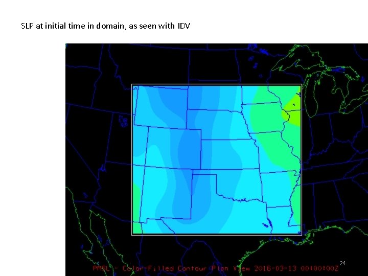
SLP at initial time in domain, as seen with IDV 24

Running real. exe and wrf. exe: Batch scripts 25

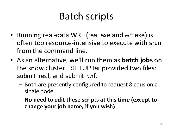
Batch scripts • Running real-data WRF (real. exe and wrf. exe) is often too resource-intensive to execute with srun from the command line. • As an alternative, we’ll run them as batch jobs on the snow cluster. SETUP. tar provided two files: submit_real, and submit_wrf. – Both are presently configured to request 8 cpus on a single node – No need to edit these scripts at this time (except to change your job name, if you wish) 26

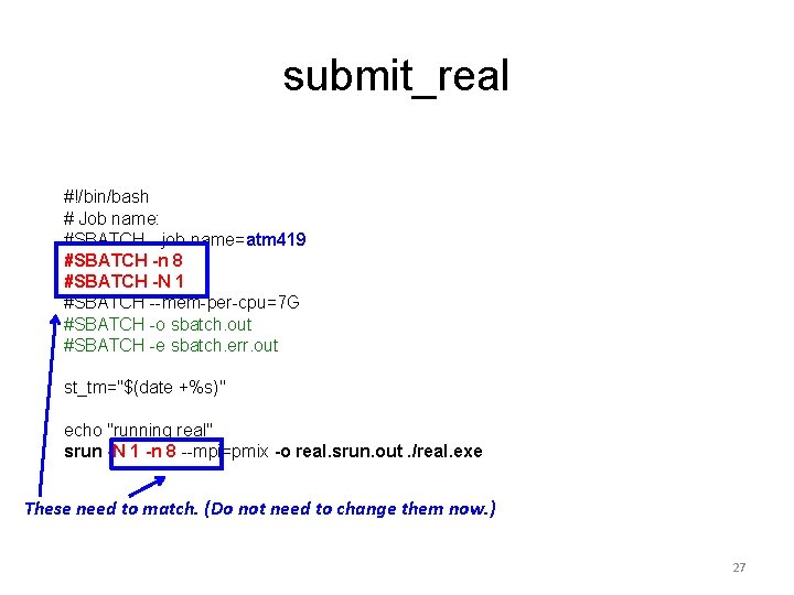
submit_real #!/bin/bash # Job name: #SBATCH --job-name=atm 419 #SBATCH -n 8 #SBATCH -N 1 #SBATCH --mem-per-cpu=7 G #SBATCH -o sbatch. out #SBATCH -e sbatch. err. out st_tm="$(date +%s)" echo "running real" srun -N 1 -n 8 --mpi=pmix -o real. srun. out. /real. exe These need to match. (Do not need to change them now. ) 27

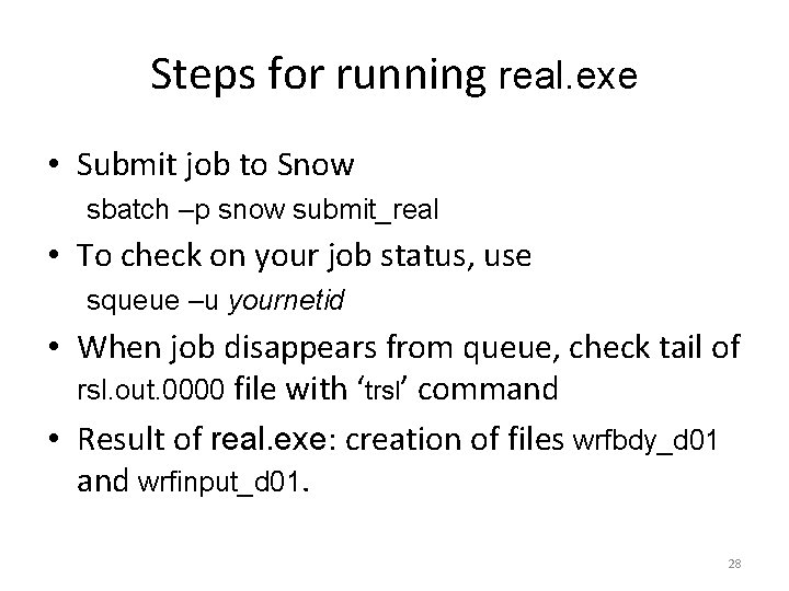
Steps for running real. exe • Submit job to Snow sbatch –p snow submit_real • To check on your job status, use squeue –u yournetid • When job disappears from queue, check tail of rsl. out. 0000 file with ‘trsl’ command • Result of real. exe: creation of files wrfbdy_d 01 and wrfinput_d 01. 28

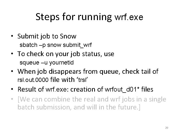
Steps for running wrf. exe • Submit job to Snow sbatch –p snow submit_wrf • To check on your job status, use squeue –u yournetid • When job disappears from queue, check tail of rsl. out. 0000 file with ‘trsl’ • Result of wrf. exe: creation of wrfout_d 01* files • [We can combine the real and wrf jobs in a single batch submission, and will in the future. ] 29

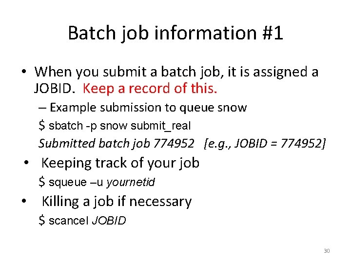
Batch job information #1 • When you submit a batch job, it is assigned a JOBID. Keep a record of this. – Example submission to queue snow $ sbatch -p snow submit_real Submitted batch job 774952 [e. g. , JOBID = 774952] • Keeping track of your job $ squeue –u yournetid • Killing a job if necessary $ scancel JOBID 30

Batch job information #2 • Usable queues: snow • Checking on queue availability $ squeue 31

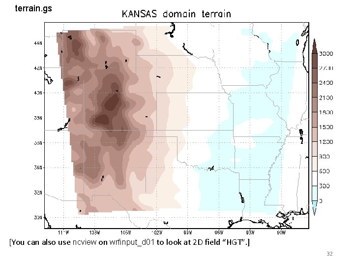
terrain. gs [You can also use ncview on wrfinput_d 01 to look at 2 D field “HGT”. ] 32

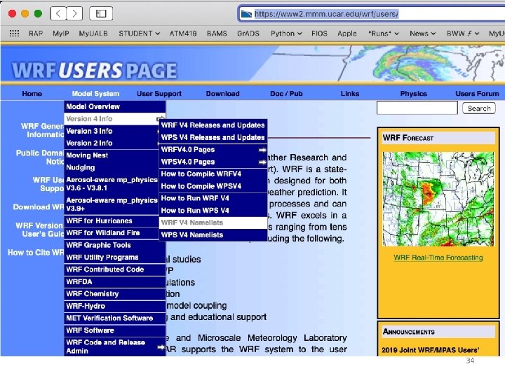
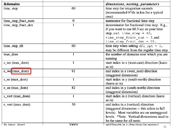
Look inside namelist. input Determine run start/end times Specify domain sizes, # of levels, time step Select model physics options …and more 33

34

35

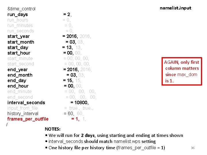
&time_control run_days run_hours run_minutes run_seconds start_year start_month start_day start_hour start_minute start_second end_year end_month end_day end_hour end_minute end_second interval_seconds input_from_file history_interval frames_per_outfile / namelist. input = 2, = 0, = 2016, = 03, = 13, = 00, 00, 00, = 2016, = 03, = 15, = 00, 00, 00, = 10800, =. true. , = 60, = 1, 1, AGAIN, only first column matters since max_dom is 1. NOTES: • We will run for 2 days, using starting and ending at times shown • interval_seconds should match namelist. wps setting • One history file per history time (frames_per_outfile = 1) 36

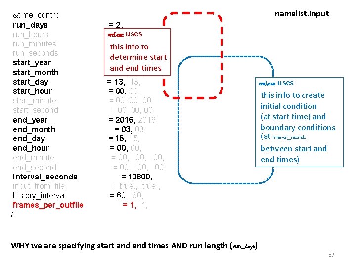
&time_control run_days run_hours run_minutes run_seconds start_year start_month start_day start_hour start_minute start_second end_year end_month end_day end_hour end_minute end_second interval_seconds input_from_file history_interval frames_per_outfile namelist. input = 2, wrf. exe = 0, uses = 0, info to this = 0, determine start = 2016, and end times = 03, = 13, = 00, 00, 00, = 2016, = 03, = 15, = 00, 00, 00, = 10800, =. true. , = 60, = 1, 1, real. exe uses this info to create initial condition (at start time) and boundary conditions (at interval_seconds between start and end times) / WHY we are specifying start and end times AND run length (run_days) 37

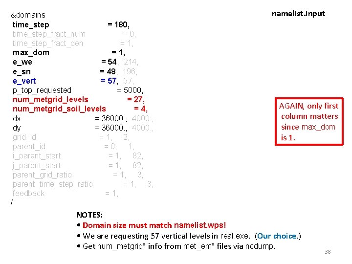
&domains time_step = 180, time_step_fract_num = 0, time_step_fract_den = 1, max_dom = 1, e_we = 54, 214, e_sn = 48, 196, e_vert = 57, p_top_requested = 5000, num_metgrid_levels = 27, num_metgrid_soil_levels = 4, dx = 36000. , 4000. , dy = 36000. , 4000. , grid_id = 1, 2, parent_id = 0, 1, i_parent_start = 1, 82, j_parent_start = 1, 82, parent_grid_ratio = 1, 3, parent_time_step_ratio = 1, 3, feedback = 1, / namelist. input AGAIN, only first column matters since max_dom is 1. NOTES: • Domain size must match namelist. wps! • We are requesting 57 vertical levels in real. exe. (Our choice. ) • Get num_metgrid* info from met_em* files via ncdump. 38

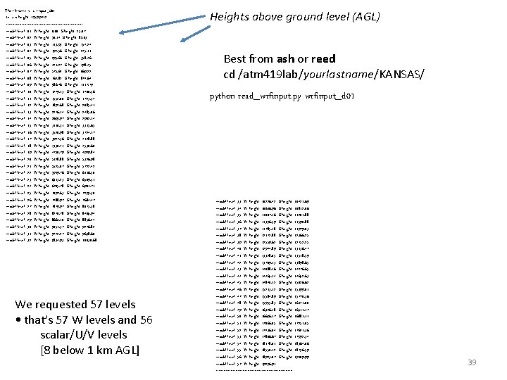
The filename is wrfinput_d 01 terrain height 1259. 9412 --------------------------------model level 01 W height 0. 00 S height 25. 07 model level 02 W height 50. 14 S height 82. 03 model level 03 W height 113. 93 S height 154. 24 model level 04 W height 194. 56 S height 245. 11 model level 05 W height 295. 66 S height 358. 46 model level 06 W height 421. 27 S height 498. 45 model level 07 W height 575. 62 S height 669. 22 model level 08 W height 762. 82 S height 874. 64 model level 09 W height 986. 46 S height 1117. 79 model level 10 W height 1249. 13 S height 1400. 56 model level 11 W height 1552. 00 S height 1723. 34 model level 12 W height 1894. 68 S height 2085. 41 model level 13 W height 2276. 14 S height 2485. 06 model level 14 W height 2693. 97 S height 2902. 14 model level 15 W height 3110. 31 S height 3315. 65 model level 16 W height 3520. 98 S height 3724. 17 model level 17 W height 3927. 36 S height 4128. 88 model level 18 W height 4330. 41 S height 4530. 60 model level 19 W height 4730. 79 S height 4929. 84 model level 20 W height 5128. 88 S height 5326. 98 model level 21 W height 5525. 07 S height 5722. 42 model level 22 W height 5919. 76 S height 6116. 50 model level 23 W height 6313. 23 S height 6509. 51 model level 24 W height 6705. 78 S height 6901. 71 model level 25 W height 7097. 63 S height 7293. 30 model level 26 W height 7488. 97 S height 7684. 47 model level 27 W height 7879. 97 S height 8075. 38 model level 28 W height 8270. 78 S height 8465. 94 model level 29 W height 8661. 10 S height 8856. 24 model level 30 W height 9051. 37 S height 9246. 82 model level 31 W height 9442. 27 S height 9638. 60 model level 32 W height 9834. 93 S height 10030. 68 We requested 57 levels • that’s 57 W levels and 56 scalar/U/V levels [8 below 1 km AGL] Heights above ground level (AGL) Best from ash or reed cd /atm 419 lab/yourlastname/KANSAS/ python read_wrfinput. py wrfinput_d 01 model level 33 W height 10226. 42 S height model level 34 W height 10616. 96 S height model level 35 W height 11007. 16 S height model level 36 W height 11396. 59 S height model level 37 W height 11785. 18 S height model level 38 W height 12172. 88 S height model level 39 W height 12559. 62 S height model level 40 W height 12944. 89 S height model level 41 W height 13328. 05 S height model level 42 W height 13709. 13 S height model level 43 W height 14088. 16 S height model level 44 W height 14465. 14 S height model level 45 W height 14840. 12 S height model level 46 W height 15213. 12 S height model level 47 W height 15584. 89 S height model level 48 W height 15955. 83 S height model level 49 W height 16326. 18 S height model level 50 W height 16696. 17 S height model level 51 W height 17066. 05 S height model level 52 W height 17436. 04 S height model level 53 W height 17806. 67 S height model level 54 W height 18178. 01 S height model level 55 W height 18550. 12 S height model level 56 W height 18923. 07 S height model level 57 W height 19296. 91 -------------------------------- 10421. 69 10812. 06 11201. 88 11590. 88 11979. 03 12366. 25 12752. 25 13136. 47 13518. 59 13898. 65 14276. 65 14652. 63 15026. 62 15399. 01 15770. 36 16141. 00 16511. 17 16881. 11 17251. 05 17621. 36 17992. 34 18364. 06 18736. 59 19109. 99 39

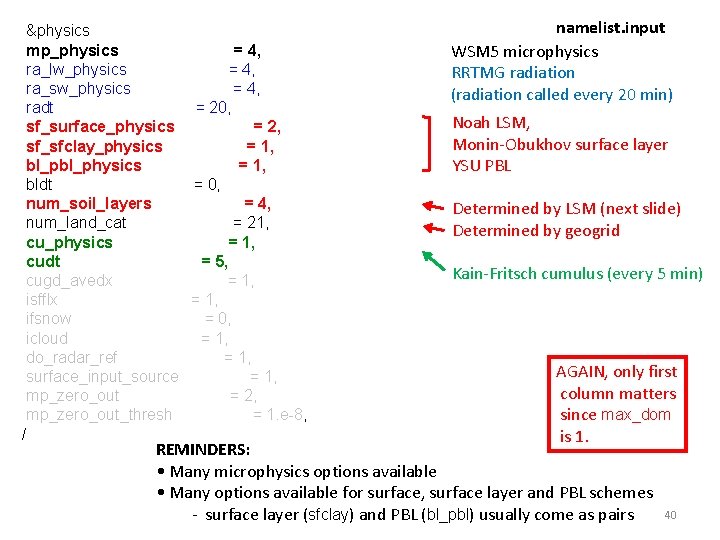
&physics mp_physics = 4, ra_lw_physics = 4, ra_sw_physics = 4, radt = 20, sf_surface_physics = 2, sf_sfclay_physics = 1, bl_physics = 1, bldt = 0, num_soil_layers = 4, num_land_cat = 21, cu_physics = 1, cudt = 5, cugd_avedx = 1, isfflx = 1, ifsnow = 0, icloud = 1, do_radar_ref = 1, surface_input_source = 1, mp_zero_out = 2, mp_zero_out_thresh = 1. e-8, / namelist. input WSM 5 microphysics RRTMG radiation (radiation called every 20 min) Noah LSM, Monin-Obukhov surface layer YSU PBL Determined by LSM (next slide) Determined by geogrid Kain-Fritsch cumulus (every 5 min) AGAIN, only first column matters since max_dom is 1. REMINDERS: • Many microphysics options available • Many options available for surface, surface layer and PBL schemes - surface layer (sfclay) and PBL (bl_pbl) usually come as pairs 40

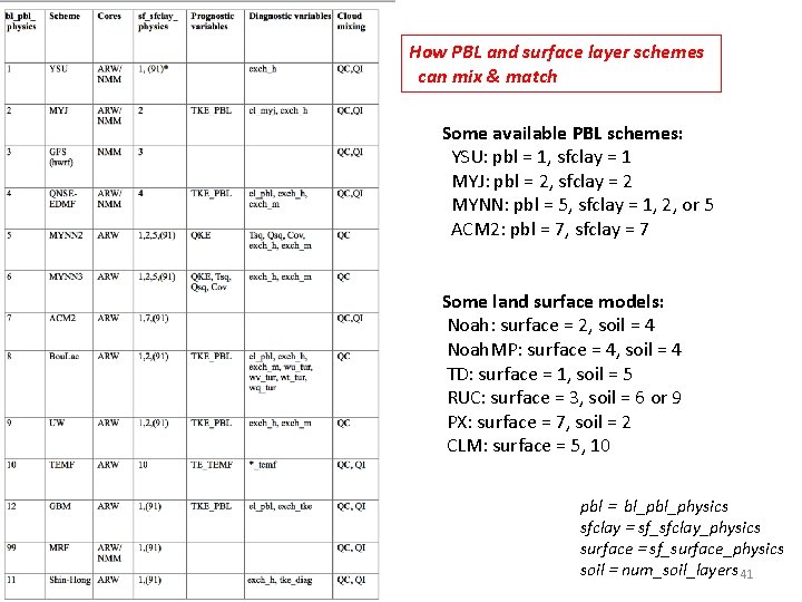
How PBL and surface layer schemes can mix & match Some available PBL schemes: YSU: pbl = 1, sfclay = 1 MYJ: pbl = 2, sfclay = 2 MYNN: pbl = 5, sfclay = 1, 2, or 5 ACM 2: pbl = 7, sfclay = 7 Some land surface models: Noah: surface = 2, soil = 4 Noah. MP: surface = 4, soil = 4 TD: surface = 1, soil = 5 RUC: surface = 3, soil = 6 or 9 PX: surface = 7, soil = 2 CLM: surface = 5, 10 pbl = bl_physics sfclay = sf_sfclay_physics surface = sf_surface_physics soil = num_soil_layers 41

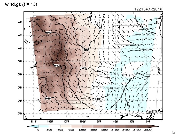
wind. gs (t = 13) 42

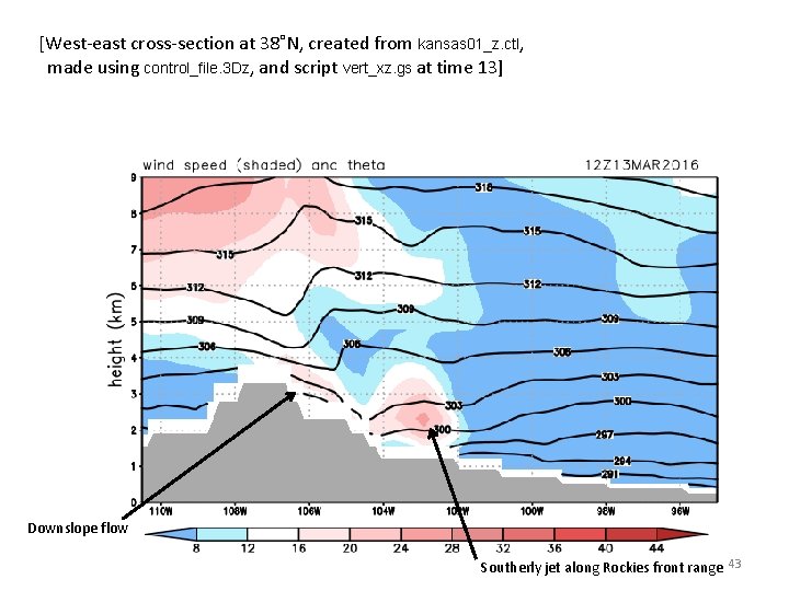
[West-east cross-section at 38˚N, created from kansas 01_z. ctl, made using control_file. 3 Dz, and script vert_xz. gs at time 13] Downslope flow Southerly jet along Rockies front range 43