Realdata WRF Verification with MET package ATM 419563

Real-data WRF: Verification with MET package ATM 419/563 Spring 2020 Fovell 1 © Copyright 2020 Robert Fovell, Univ. at Albany, SUNY, rfovell@albany. edu

Terms AGL = above (local) ground level MSL = above mean sea level ASOS = Automated Surface Observing System MET = Model Evaluation Tools package MADIS = Meteorological Assimilation Data Ingest System • METAR = Meteorological Terminal Aviation Routine Weather Report (an obs data format) • • • 2

References • MET Users Guide (version 6. 0) (PDF) – Not the most recent version • UPP Users Guide (version 4) (PDF) • ASOS home page • MADIS data web portal MET has advanced to version 8. 1 at this time 3

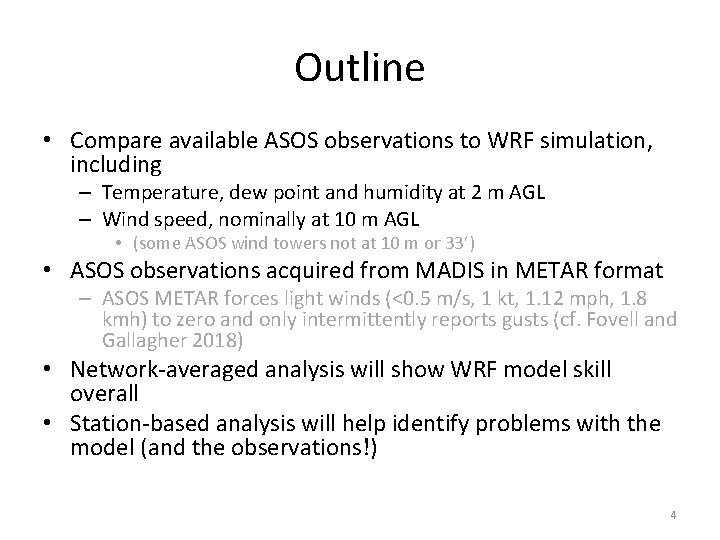
Outline • Compare available ASOS observations to WRF simulation, including – Temperature, dew point and humidity at 2 m AGL – Wind speed, nominally at 10 m AGL • (some ASOS wind towers not at 10 m or 33’) • ASOS observations acquired from MADIS in METAR format – ASOS METAR forces light winds (<0. 5 m/s, 1 kt, 1. 12 mph, 1. 8 kmh) to zero and only intermittently reports gusts (cf. Fovell and Gallagher 2018) • Network-averaged analysis will show WRF model skill overall • Station-based analysis will help identify problems with the model (and the observations!) 4

Part 1: Network-averaged analysis See script for required actions 5

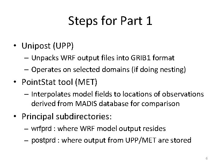
Steps for Part 1 • Unipost (UPP) – Unpacks WRF output files into GRIB 1 format – Operates on selected domains (if doing nesting) • Point. Stat tool (MET) – Interpolates model fields to locations of observations derived from MADIS database for comparison • Principal subdirectories: – wrfprd : where WRF model output resides – postprd : where output from UPP/MET are stored 6

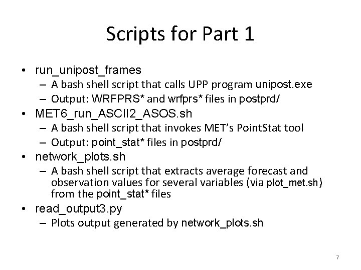
Scripts for Part 1 • run_unipost_frames – A bash shell script that calls UPP program unipost. exe – Output: WRFPRS* and wrfprs* files in postprd/ • MET 6_run_ASCII 2_ASOS. sh – A bash shell script that invokes MET’s Point. Stat tool – Output: point_stat* files in postprd/ • network_plots. sh – A bash shell script that extracts average forecast and observation values for several variables (via plot_met. sh) from the point_stat* files • read_output 3. py – Plots output generated by network_plots. sh 7

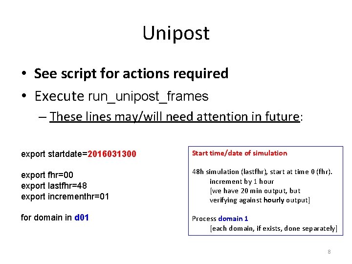
Unipost • See script for actions required • Execute run_unipost_frames – These lines may/will need attention in future: export startdate=2016031300 Start time/date of simulation export fhr=00 export lastfhr=48 export incrementhr=01 48 h simulation (lastfhr), start at time 0 (fhr). increment by 1 hour [we have 20 min output, but verifying against hourly output] for domain in d 01 Process domain 1 [each domain, if exists, done separately] 8

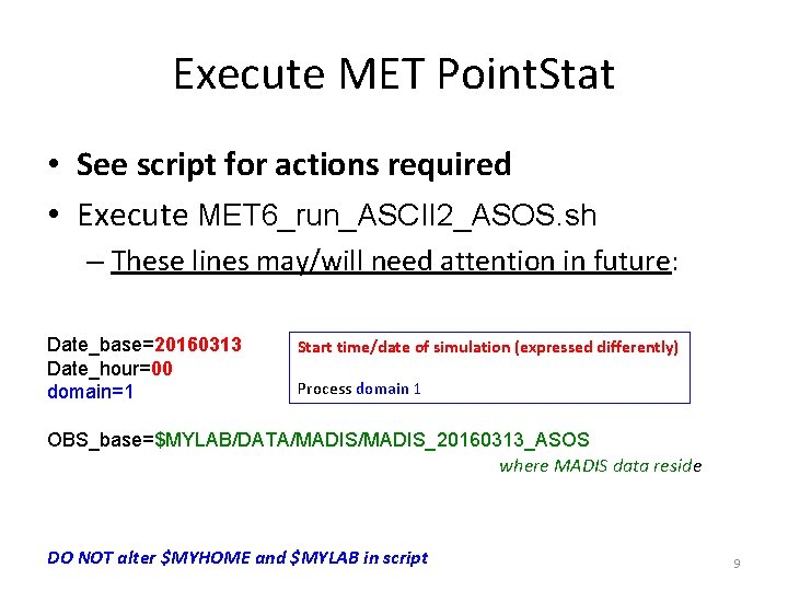
Execute MET Point. Stat • See script for actions required • Execute MET 6_run_ASCII 2_ASOS. sh – These lines may/will need attention in future: Date_base=20160313 Date_hour=00 domain=1 Start time/date of simulation (expressed differently) Process domain 1 OBS_base=$MYLAB/DATA/MADIS_20160313_ASOS where MADIS data reside DO NOT alter $MYHOME and $MYLAB in script 9

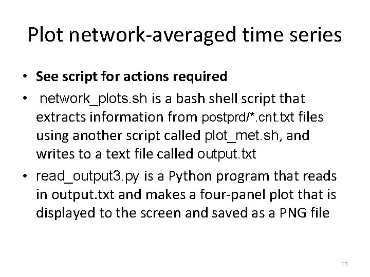
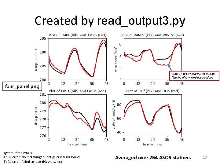
Plot network-averaged time series • See script for actions required • network_plots. sh is a bash shell script that extracts information from postprd/*. cnt. txt files using another script called plot_met. sh, and writes to a text file called output. txt • read_output 3. py is a Python program that reads in output. txt and makes a four-panel plot that is displayed to the screen and saved as a PNG file 10

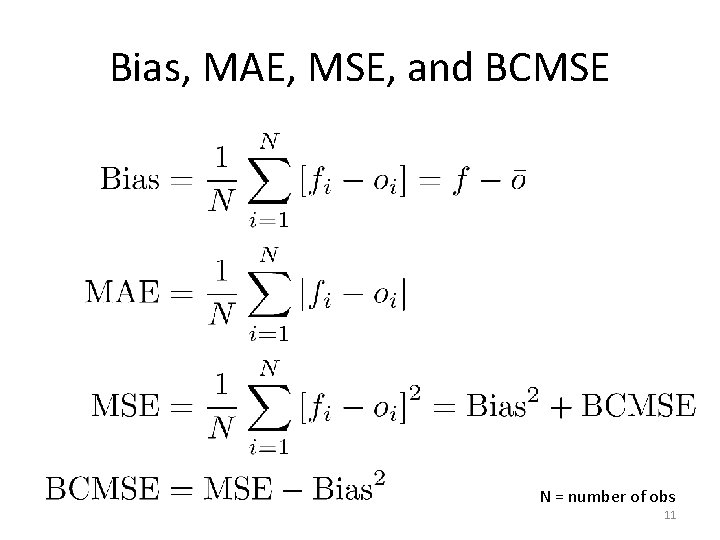
Bias, MAE, MSE, and BCMSE N = number of obs 11

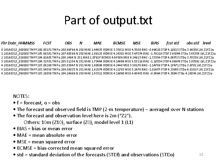
Part of output. txt Fhr Date_HHMMSS FCST OBS N MAE BCMSE BIAS fcst std obs std level 0 20160313_000000 TMPf 288. 00171 TMPo 288. 99799 N 250 MAE 1. 46435 BCMSE 3. 35822 MSE 4. 3508 BIAS -0. 99628 STDf 4. 10823 STDo 3. 99308 LVL Z 2 f Z 2 o 1 20160313_010000 TMPf 285. 69381 TMPo 287. 48599 N 250 MAE 2. 09225 BCMSE 4. 26382 MSE 7. 47574 BIAS -1. 79218 STDf 3. 93064 STDo 3. 65356 LVL Z 2 f Z 2 o 2 20160313_020000 TMPf 284. 91605 TMPo 286. 2496 N 251 MAE 1. 87927 BCMSE 4. 47089 MSE 6. 24923 BIAS -1. 33354 STDf 4. 06753 STDo 3. 78339 LVL Z 2 f Z 2 o 3 20160313_030000 TMPf 284. 32701 TMPo 285. 51254 N 251 MAE 1. 73464 BCMSE 4. 14669 MSE 5. 55219 BIAS -1. 18554 STDf 4. 09976 STDo 3. 87092 LVL Z 2 f Z 2 o 4 20160313_040000 TMPf 283. 88289 TMPo 285. 03047 N 251 MAE 1. 68696 BCMSE 4. 2448 MSE 5. 56176 BIAS -1. 14759 STDf 4. 17471 STDo 3. 8701 LVL Z 2 f Z 2 o 5 20160313_050000 TMPf 283. 54558 TMPo 284. 56035 N 251 MAE 1. 62574 BCMSE 4. 21783 MSE 5. 2476 BIAS -1. 01477 STDf 4. 33065 STDo 4. 02827 LVL Z 2 f Z 2 o 6 20160313_060000 TMPf 283. 28059 TMPo 284. 14999 N 250 MAE 1. 63312 BCMSE 4. 19868 MSE 4. 95455 BIAS -0. 8694 STDf 4. 3884 STDo 4. 28034 LVL Z 2 f Z 2 o NOTES: • f = forecast, o = obs • The forecast and observed field is TMP (2 -m temperature) – averaged over N stations • The forecast and observation level here is 2 m (“Z 2”). Others: 10 m (Z 10), surface (Z 0), model level 1 (L 1) • BIAS = bias or mean error • MAE = mean absolute error • MSE = mean squared error • BCMSE = bias-corrected mean squared error 12 • std = standard deviation of the forecasts (STDf) and observations (STDo)

Created by read_output 3. py Some of this is likely due to METAR filtering of low wind observations four_panel. png Ignore these errors… lib. GL error: No matching fb. Configs or visuals found lib. GL error: failed to load driver: swrast Averaged over 254 ASOS stations 13

Notes for future applications • The run_unipost_frames script is set up for a WRF run with multiple output times written to a single wrfout file. A different version of the script will be used for experiments in which each output time is written to a unique wrfout file. • The Point. Stat configuration file (Point. Stat. Config. ATM 419. NEAREST. ASOS. NOGUSTS. SUBSET) called in the MET script controls which variables are selected for verification, how they are paired, and how data are interpolated. This file needs to be copied/altered if you wish to include other fields (like SLP, gusts) in your verification. • The python plotting script requires modification if your analysis interval is not hourly or variables need to be added. Also, axis scales are specified and may need to be revised for other cases. 14

Part 2: Station-based analysis of 10 m wind speed and 2 m temperature See script for required actions 15

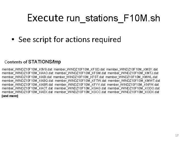
Scripts for Part 2 • run_stations_*. sh – Bash shell scripts that call a Perl script that combs through point_stat* files in postprd/ for individual stations – Output: Station by station files like member_WINDZ 10 F 10 M_KBMQ. dat in directory STATIONS/tmp • sum_and_average_*. sh – Bash shell scripts that call a Perl script that reads through files in directory STATIONS/tmp – Output: input_for_grads file • grads_plot. sh – A bash shell script that calls a Perl script to create a Gr. ADS script for plotting from contents of input_for_grads – Output: stations. gs 16

Execute run_stations_F 10 M. sh • See script for actions required Contents of STATIONS/tmp member_WINDZ 10 F 10 M_K 9 V 9. dat member_WINDZ 10 F 10 M_KFSD. dat member_WINDZ 10 F 10 M_KMSY. dat member_WINDZ 10 F 10 M_KAAO. dat member_WINDZ 10 F 10 M_KFSM. dat member_WINDZ 10 F 10 M_KMTJ. dat member_WINDZ 10 F 10 M_KABI. dat member_WINDZ 10 F 10 M_KFST. dat member_WINDZ 10 F 10 M_KMWL. dat member_WINDZ 10 F 10 M_KABQ. dat member_WINDZ 10 F 10 M_KFTW. dat member_WINDZ 10 F 10 M_KMWT. dat member_WINDZ 10 F 10 M_KABR. dat member_WINDZ 10 F 10 M_KFYV. dat member_WINDZ 10 F 10 M_KNFW. dat member_WINDZ 10 F 10 M_KACT. dat member_WINDZ 10 F 10 M_KGAG. dat member_WINDZ 10 F 10 M_KODO. dat member_WINDZ 10 F 10 M_KAEX. dat member_WINDZ 10 F 10 M_KGCC. dat member_WINDZ 10 F 10 M_KODX. dat [and more] 17

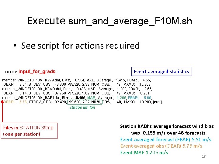
Execute sum_and_average_F 10 M. sh • See script for actions required more input_for_grads Event-averaged statistics member_WINDZ 10 F 10 M_K 9 V 9. dat, Bias: , 0. 904, MAE, Average: , OBAR: , 3. 64, STDEV_OBS: , 43. 800, -99. 320, 2. 33, NUM_OBS, member_WINDZ 10 F 10 M_KAAO. dat, Bias: , -0. 486, MAE, Average: , OBAR: , 3. 14, STDEV_OBS: , 37. 750, -97. 220, 1. 62, NUM_OBS, member_WINDZ 10 F 10 M_KABI. dat, Bias: , -0. 155, MAE, Average: , OBAR: , 5. 76, STDEV_OBS: , 32. 420, -99. 680, 2. 32, NUM_OBS, 1. 415, FBAR: , 4. 55, 49, MAXO: , 10. 803, 1. 283, FBAR: , 2. 65, 49, MAXO: , 8. 231, 1. 206, FBAR: , 5. 60, 48, MAXO: , 10. 289, [etc. ] station lat, lon Files in STATIONS/tmp (one per station) Station KABI’s average forecast wind bias was -0. 155 m/s over 48 forecasts Event-averaged forecast (FBAR) 5. 51 m/s Event-averaged obs (OBAR) 5. 76 m/s Event MAE 1. 206 m/s 18

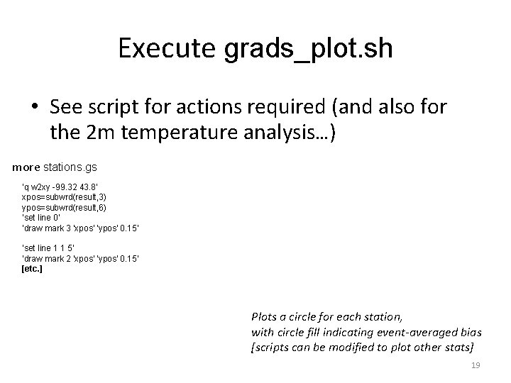
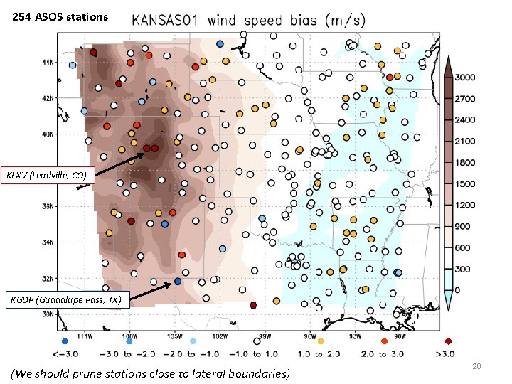
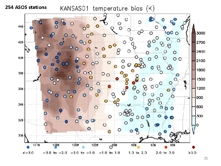
Execute grads_plot. sh • See script for actions required (and also for the 2 m temperature analysis…) more stations. gs 'q w 2 xy -99. 32 43. 8' xpos=subwrd(result, 3) ypos=subwrd(result, 6) 'set line 0' 'draw mark 3 'xpos' 'ypos' 0. 15' 'set line 1 1 5' 'draw mark 2 'xpos' 'ypos' 0. 15’ [etc. ] Plots a circle for each station, with circle fill indicating event-averaged bias [scripts can be modified to plot other stats] 19

254 ASOS stations KLXV (Leadville, CO) KGDP (Guadalupe Pass, TX) (We should prune stations close to lateral boundaries) 20

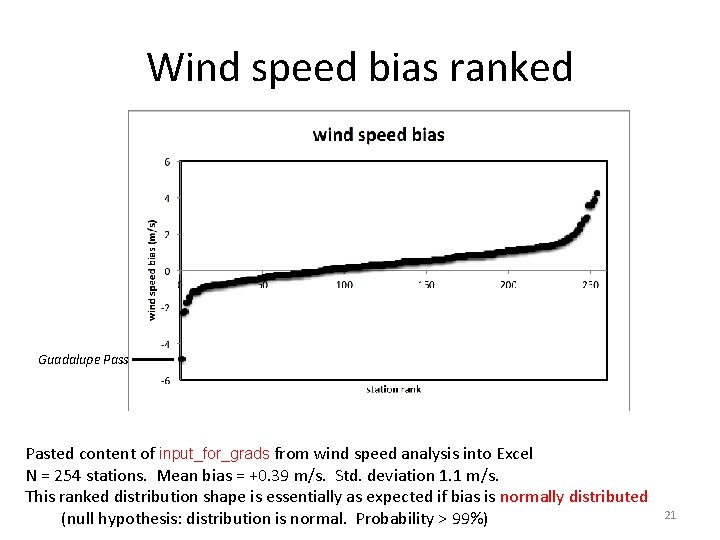
Wind speed bias ranked Guadalupe Pass Pasted content of input_for_grads from wind speed analysis into Excel N = 254 stations. Mean bias = +0. 39 m/s. Std. deviation 1. 1 m/s. This ranked distribution shape is essentially as expected if bias is normally distributed (null hypothesis: distribution is normal. Probability > 99%) 21

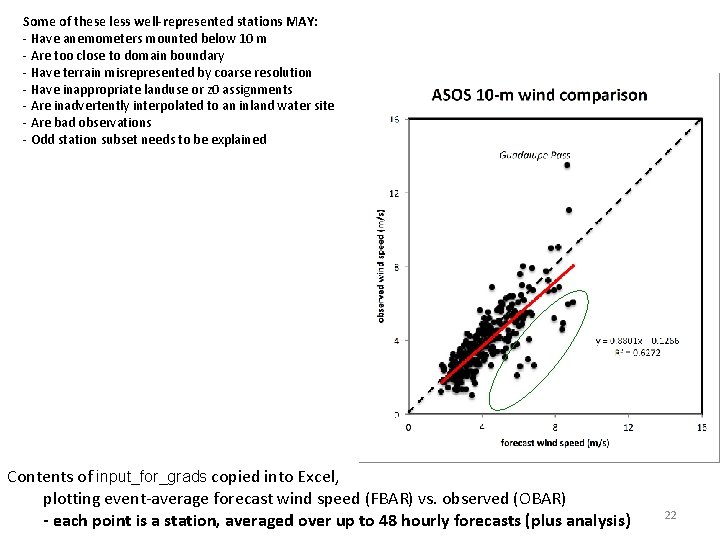
Some of these less well-represented stations MAY: - Have anemometers mounted below 10 m - Are too close to domain boundary - Have terrain misrepresented by coarse resolution - Have inappropriate landuse or z 0 assignments - Are inadvertently interpolated to an inland water site - Are bad observations - Odd station subset needs to be explained Contents of input_for_grads copied into Excel, plotting event-average forecast wind speed (FBAR) vs. observed (OBAR) - each point is a station, averaged over up to 48 hourly forecasts (plus analysis) 22

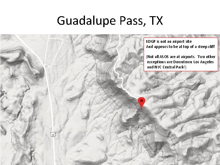
Guadalupe Pass, TX KDGP is not an airport site And appears to be at top of a steep cliff (Not all ASOS are at airports. Two other exceptions are Downtown Los Angeles and NYC Central Park!) 23

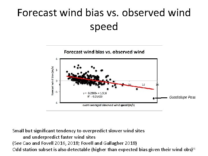
Forecast wind bias vs. observed wind speed Guadalupe Pass Small but significant tendency to overpredict slower wind sites and underpredict faster wind sites (See Cao and Fovell 2016, 2018; Fovell and Gallagher 2018) Odd station subset is also detectable (higher than expected bias given their wind obs)24

254 ASOS stations 25

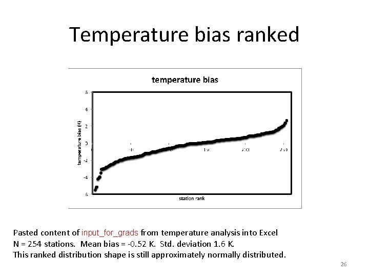
Temperature bias ranked Pasted content of input_for_grads from temperature analysis into Excel N = 254 stations. Mean bias = -0. 52 K. Std. deviation 1. 6 K. This ranked distribution shape is still approximately normally distributed. 26

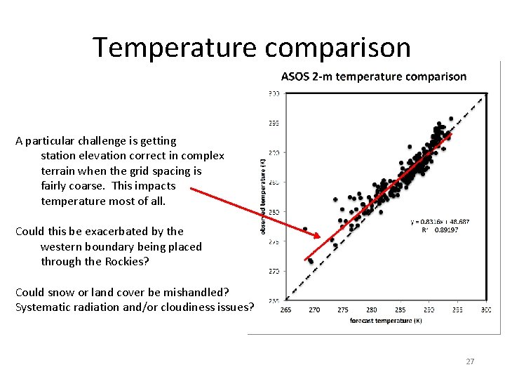
Temperature comparison A particular challenge is getting station elevation correct in complex terrain when the grid spacing is fairly coarse. This impacts temperature most of all. Could this be exacerbated by the western boundary being placed through the Rockies? Could snow or land cover be mishandled? Systematic radiation and/or cloudiness issues? 27

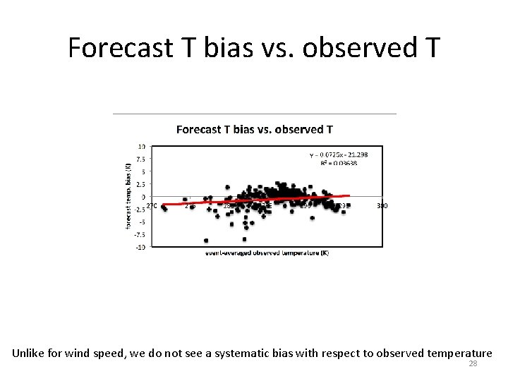
Forecast T bias vs. observed T Unlike for wind speed, we do not see a systematic bias with respect to observed temperature 28