Quantum Computing Instructors Frank Mueller Patrick Dreher Greg

Quantum Computing Instructors: Frank Mueller, Patrick Dreher, Greg Byrd TA: Mond Ibrahim CSC 591 -050/ECE 592 -050 Fall 2019 1

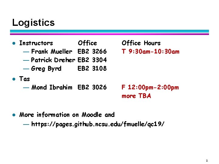
Logistics l l l Instructors — Frank Mueller — Patrick Dreher — Greg Byrd Office EB 2 3266 EB 2 3304 EB 2 3108 Tas — Mond Ibrahim EB 2 3026 Office Hours T 9: 30 am-10: 30 am F 12: 00 pm-2: 00 pm more TBA More information on Moodle and — https: //pages. github. ncsu. edu/fmuelle/qc 19/ 2

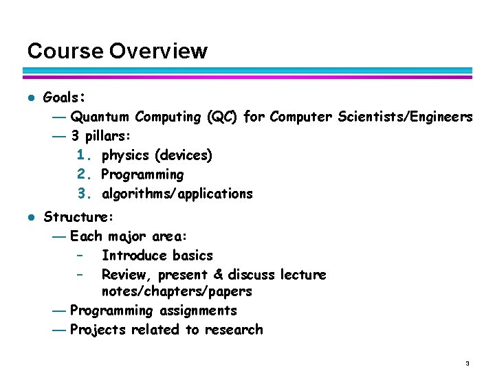
Course Overview l l Goals: — Quantum Computing (QC) for Computer Scientists/Engineers — 3 pillars: 1. physics (devices) 2. Programming 3. algorithms/applications Structure: — Each major area: – Introduce basics – Review, present & discuss lecture notes/chapters/papers — Programming assignments — Projects related to research 3

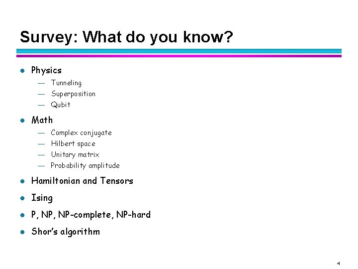
Survey: What do you know? l Physics — Tunneling — Superposition — Qubit l Math — Complex conjugate — Hilbert space — Unitary matrix — Probability amplitude l Hamiltonian and Tensors l Ising l P, NP-complete, NP-hard l Shor’s algorithm 4

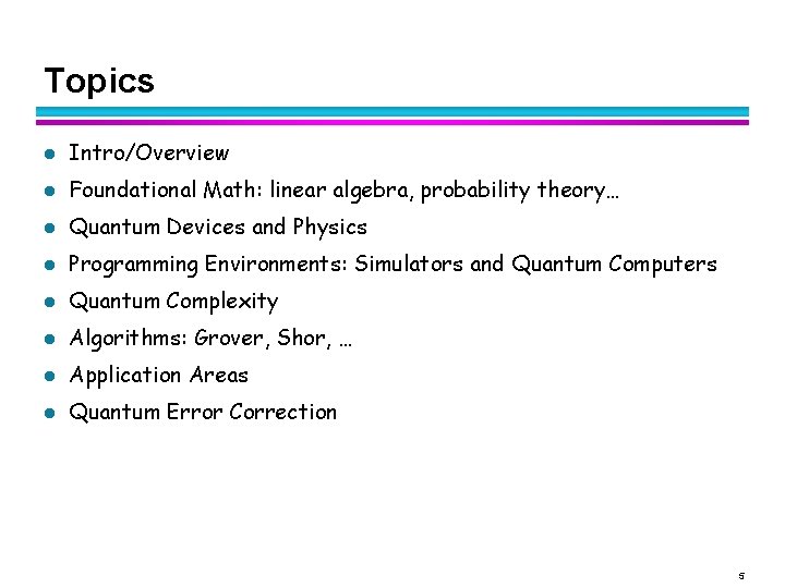
Topics l Intro/Overview l Foundational Math: linear algebra, probability theory… l Quantum Devices and Physics l Programming Environments: Simulators and Quantum Computers l Quantum Complexity l Algorithms: Grover, Shor, … l Application Areas l Quantum Error Correction 5

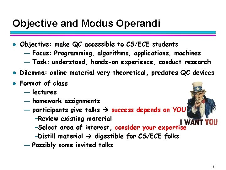
Objective and Modus Operandi l l l Objective: make QC accessible to CS/ECE students — Focus: Programming, algorithms, applications, machines — Task: understand, hands-on experience, conduct research Dilemma: online material very theoretical, predates QC devices Format of class — lectures — homework assignments — participants give talks success depends on YOU –Review existing material –Select area of interest, consider your expertise –Distill material digestible for CS/ECE folks — Possibly some invited talks 6

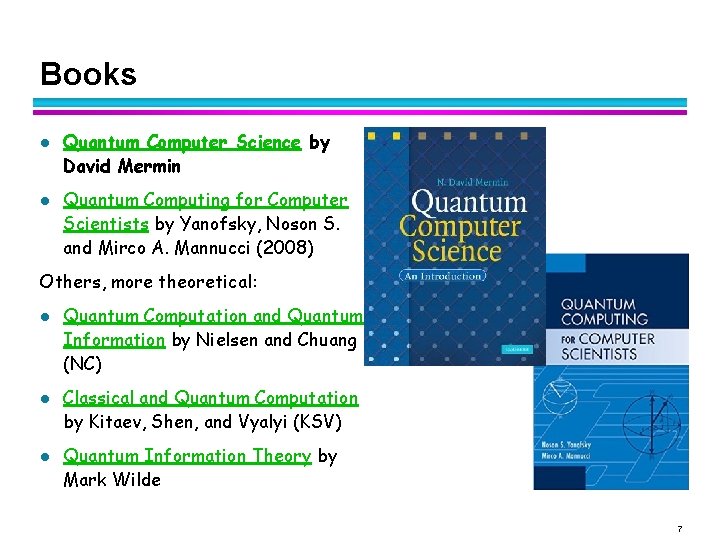
Books l l Quantum Computer Science by David Mermin Quantum Computing for Computer Scientists by Yanofsky, Noson S. and Mirco A. Mannucci (2008) Others, more theoretical: l l l Quantum Computation and Quantum Information by Nielsen and Chuang (NC) Classical and Quantum Computation by Kitaev, Shen, and Vyalyi (KSV) Quantum Information Theory by Mark Wilde 7

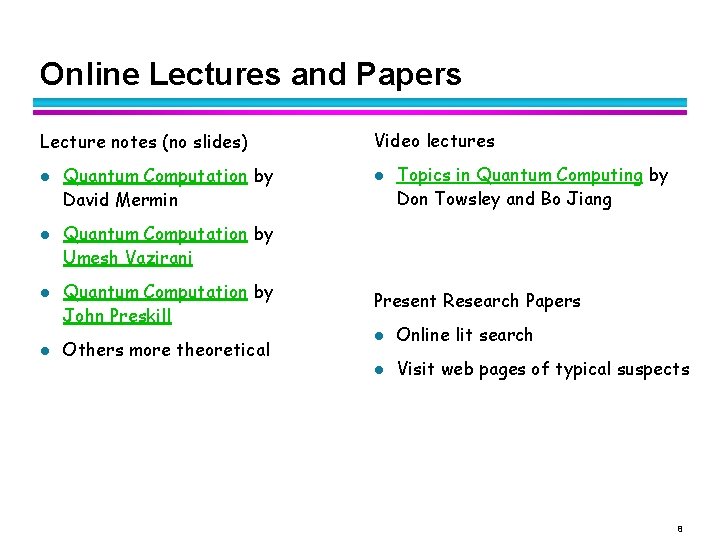
Online Lectures and Papers Lecture notes (no slides) l l Quantum Computation by David Mermin Video lectures l Topics in Quantum Computing by Don Towsley and Bo Jiang Quantum Computation by Umesh Vazirani Quantum Computation by John Preskill Others more theoretical Present Research Papers l Online lit search l Visit web pages of typical suspects 8

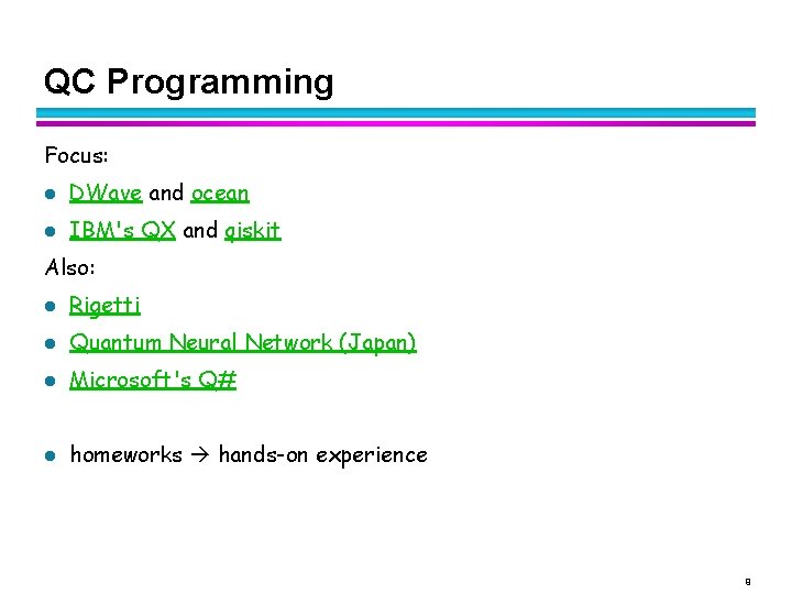
QC Programming Focus: l DWave and ocean l IBM's QX and qiskit Also: l Rigetti l Quantum Neural Network (Japan) l Microsoft's Q# l homeworks hands-on experience 9

Grading l Programming assignments / project 50% (if applicable) l Exams/Tests 40% (midterm+final) l Presentation 10% l See on-line syllabus and policies 10

Today l Intro to QC — Slides adopted from Scott Pakin (LANL) 11

Quantum Computing Basics [some slides originate from Scott Pakin (LANL)] 12

Outline l Performance potential of quantum computing l Quantum annealing l Case study: D-Wave quantum annealers l How to program a quantum annealer l Example: Map coloring 13

What problems can quantum computers solve fast? l What “flavor” of quantum are we referring to? l What exactly is a computer? l What do we mean by solve? l What is considered fast in this context? 14

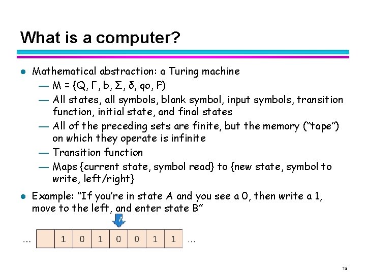
What is a computer? l l Mathematical abstraction: a Turing machine — M = {Q, Γ, b, Σ, δ, qo, F) — All states, all symbols, blank symbol, input symbols, transition function, initial state, and final states — All of the preceding sets are finite, but the memory (“tape”) on which they operate is infinite — Transition function — Maps {current state, symbol read} to {new state, symbol to write, left/right} Example: “If you’re in state A and you see a 0, then write a 1, move to the left, and enter state B” 15

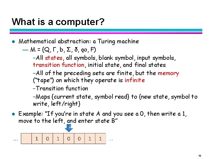
What is a computer? l l Mathematical abstraction: a Turing machine — M = {Q, Γ, b, Σ, δ, qo, F) –All states, all symbols, blank symbol, input symbols, transition function, initial state, and final states –All of the preceding sets are finite, but the memory (“tape”) on which they operate is infinite –Transition function –Maps {current state, symbol read} to {new state, symbol to write, left/right} Example: “If you’re in state A and you see a 0, then write a 1, move to the left, and enter state B” 16

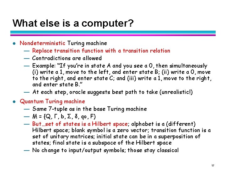
What else is a computer? l l Nondeterministic Turing machine — Replace transition function with a transition relation — Contradictions are allowed — Example: “If you’re in state A and you see a 0, then simultaneously (i) write a 1, move to the left, and enter state B; (ii) write a 0, move to the right, and enter state C; and (iii) write a 1, move to the right, and enter state B. ” — At each step, oracle suggests best path to take (unrealistic!) Quantum Turing machine — Same 7 -tuple as in the base Turing machine — M = {Q, Γ, b, Σ, δ, qo, F) — But…set of states is a Hilbert space; alphabet is a (different) Hilbert space; blank symbol is a zero vector; transition function is a set of unitary matrices; initial state can be in a superposition of states; final state is a subspace of the Hilbert space — No change to input/output symbols; those stay classical 17

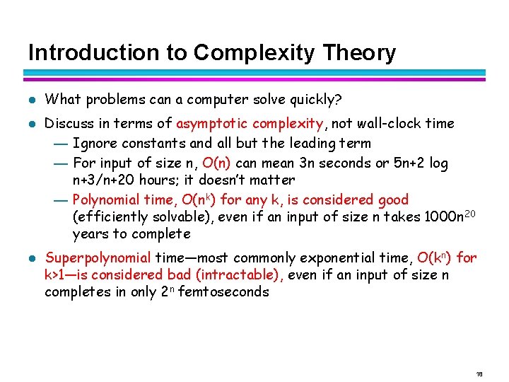
Introduction to Complexity Theory l l l What problems can a computer solve quickly? Discuss in terms of asymptotic complexity, not wall-clock time — Ignore constants and all but the leading term — For input of size n, O(n) can mean 3 n seconds or 5 n+2 log n+3/n+20 hours; it doesn’t matter — Polynomial time, O(nk) for any k, is considered good (efficiently solvable), even if an input of size n takes 1000 n 20 years to complete Superpolynomial time—most commonly exponential time, O(kn) for k>1—is considered bad (intractable), even if an input of size n completes in only 2 n femtoseconds 18

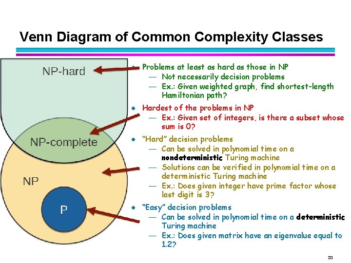
Venn Diagram of Common Complexity Classes l l Problems at least as hard as those in NP — Not necessarily decision problems — Ex. : Given weighted graph, find shortest-length Hamiltonian path? Hardest of the problems in NP — Ex. : Given set of integers, is there a subset whose sum is 0? “Hard” decision problems — Can be solved in polynomial time on a nondeterministic Turing machine — Solutions can be verified in polynomial time on a deterministic Turing machine — Ex. : Does given integer have prime factor whose last digit is 3? “Easy” decision problems — Can be solved in polynomial time on a deterministic Turing machine — Ex. : Does given matrix have an eigenvalue equal to 1. 2? 20

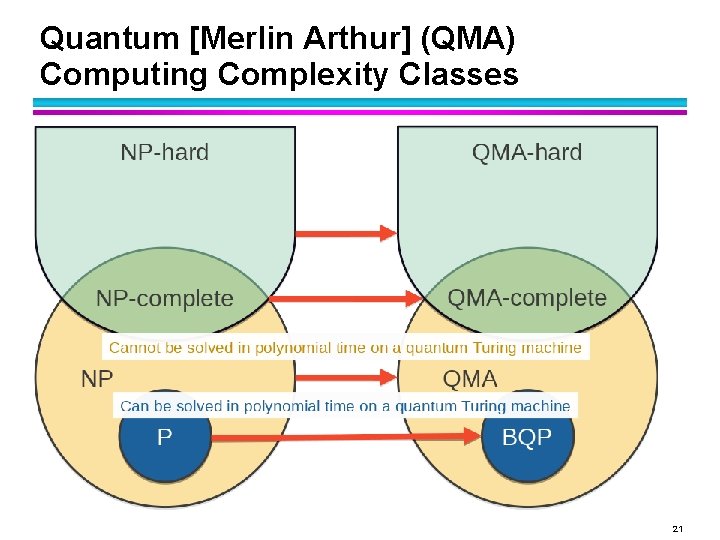
Quantum [Merlin Arthur] (QMA) Computing Complexity Classes 21

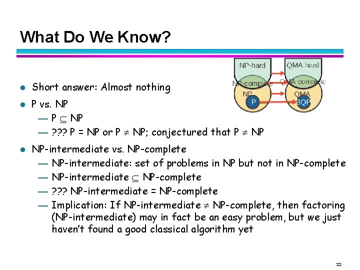
What Do We Know? l l l Short answer: Almost nothing P vs. NP — P NP — ? ? ? P = NP or P NP; conjectured that P NP NP-intermediate vs. NP-complete — NP-intermediate: set of problems in NP but not in NP-complete — NP-intermediate NP-complete — ? ? ? NP-intermediate = NP-complete — Implication: If NP-intermediate NP-complete, then factoring (NP-intermediate) may in fact be an easy problem, but we just haven’t found a good classical algorithm yet 22

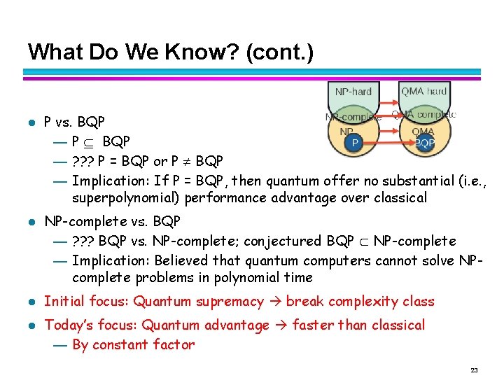
What Do We Know? (cont. ) l l P vs. BQP — P BQP — ? ? ? P = BQP or P BQP — Implication: If P = BQP, then quantum offer no substantial (i. e. , superpolynomial) performance advantage over classical NP-complete vs. BQP — ? ? ? BQP vs. NP-complete; conjectured BQP NP-complete — Implication: Believed that quantum computers cannot solve NPcomplete problems in polynomial time Initial focus: Quantum supremacy break complexity class Today’s focus: Quantum advantage faster than classical — By constant factor 23

Quantum Architectures 1. Quantum annealer (D-Wave) — Specialized: optimization problems find lowest energy level — Uses tunneling and entanglement — Better than classical? unknown, maybe significant speedup 2. Approximate quantum [gate] computer (IBM Q, Regetti, Ion. Q…) — More general: optimization, quantum chemistry, machine learning — Superposition, entanglement — Better than classical? likely, sign. Speedup: “advantage” 3. Fault-tolerant quantum computer (in “some years” from now) — Deals w/ errors (noise) algorithmically — Most general: crypto, search, and any of the above ones — Need 1000 physical qubits per virtual (“error-free”) qubit — Better than classical? proved theoretically: “supremacy” 25

Quantum Algorithms (Gate Model) l l Key concepts — N classical bits go in, N classical bits come out — Can operate on all 2 N possibilities in between — Requirement: Computation must be reversible (not a big deal in practice) — Main challenge: You get only one measurement; how do you know to measure the answer you’re looking for? — High-level approach: Quantum states based on complexvalued probability amplitudes, not probabilities—can sum to 0 to make a possibility go away — Very difficult in practice Google “quantum algorithm zoo” 60 algorithms known to date — Based on only a handful of building blocks — Each requires substantial cleverness; not much in the way of a standard approach 26

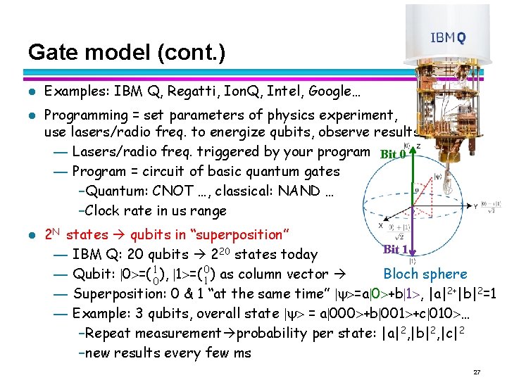
Gate model (cont. ) l l l Examples: IBM Q, Regatti, Ion. Q, Intel, Google… Programming = set parameters of physics experiment, use lasers/radio freq. to energize qubits, observe results — Lasers/radio freq. triggered by your program Bit 0 — Program = circuit of basic quantum gates –Quantum: CNOT …, classical: NAND … –Clock rate in us range 2 N states qubits in “superposition” Bit 1 — IBM Q: 20 qubits 220 states today — Qubit: 0 =( 10 ), 1 =( 01 ) as column vector Bloch sphere — Superposition: 0 & 1 “at the same time” =a 0 +b 1 , |a|2+|b|2=1 — Example: 3 qubits, overall state = a 000 +b 001 +c 010 … –Repeat measurement probability per state: |a|2, |b|2, |c|2 –new results every few ms 27

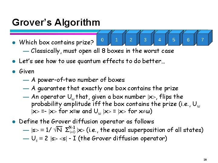
Grover’s Algorithm l l Which box contains prize? — Classically, must open all 8 boxes in the worst case Let’s see how to use quantum effects to do better… Given — A power-of-two number of boxes — A guarantee that exactly one box contains the prize — An operator Uω that, given a box number x , flips the probability amplitude iff the box contains the prize (i. e. , U ω x =- x for x=w and Uω x = x for x ω) Define the Grover diffusion operator as follows N-1 — s ≡ 1/ N Σi=0 x (i. e. , the equal superposition of all states) — Us ≡ 2 s s - I (the Grover diffusion operator) 28

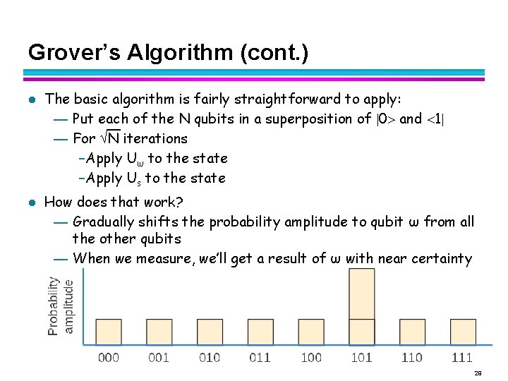
Grover’s Algorithm (cont. ) l l The basic algorithm is fairly straightforward to apply: — Put each of the N qubits in a superposition of 0 and 1 — For N iterations –Apply Uω to the state –Apply Us to the state How does that work? — Gradually shifts the probability amplitude to qubit ω from all the other qubits — When we measure, we’ll get a result of ω with near certainty 29

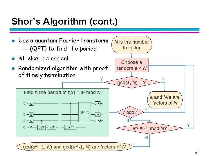
Shor’s Algorithm l l Factor 1, 274, 093, 332, 123, 426, 680, 869 into product of 2 primes — Okay, it’s 135, 763, 451, 261× 9, 384, 656, 329 Observations — Given that N is the product of two primes, p and q — Given some a that is divisible by neither p nor q — Then sequence {a 1 mod N, a 2 mod N, a 3 mod N, a 4 mod N, a 5 mod N, …} will repeat every r elements (sequence’s period) — As Euler discovered (~1760), r always divides (p− 1) (q− 1) Example — Let a be 2 and N be 15 (=3× 5), then: — ax mod N = {2, 4, 8, 1, 2, 4, 8, 1 …} r is 4 — Lo and behold, 4 divides (3− 1) (5− 1)=8 Approach — Once period, r, know, not too hard to find N’s prime factors p, q — But finding r is very time-consuming…for classical computer 30

Shor’s Algorithm (cont. ) l l l Use a quantum Fourier transform — (QFT) to find the period All else is classical Randomized algorithm with proof of timely termination 31