Product Markets and National Output Chapter 12 Discussion

Product Markets and National Output Chapter 12

Discussion Topics üCircular flow of payments üComposition and measurement of gross domestic product üConsumption, saving and investment üEquilibrium national income and output

Partial vs General Equilibrium ü Discussion of market outcomes in the preceding chapters was conducted within a partial equilibrium framework ü Partial Equilibrium – focus on a single market, assuming everything else remains constant ü General Equilibrium – focus on all markets in the economy; all markets are interdependent ü Objectives of Chapter ü Illustrate how businesses and households are linked through resource and product markets ü Discuss the composition and measurement of national output

Circular Flow Diagram for the General Economy

We can measure macroeconomic activity in either resource markets or product markets. Page 224

Four major sectors in the U. S. economy… Page 224

Businesses are net borrowers in financial markets while households are net savers… Page 224

Government receives net inflows of taxes from businesses and households and is a net borrower in financial markets… Page 224

Businesses make investment expenditures, Governments make expenditures, and Households make consumption expenditures Page 224

Businesses receive funds from total expenditures in product markets while households, who own businesses, receive wages, rents, interest and business in resource markets profits where they provide labor and capital services… Page 224

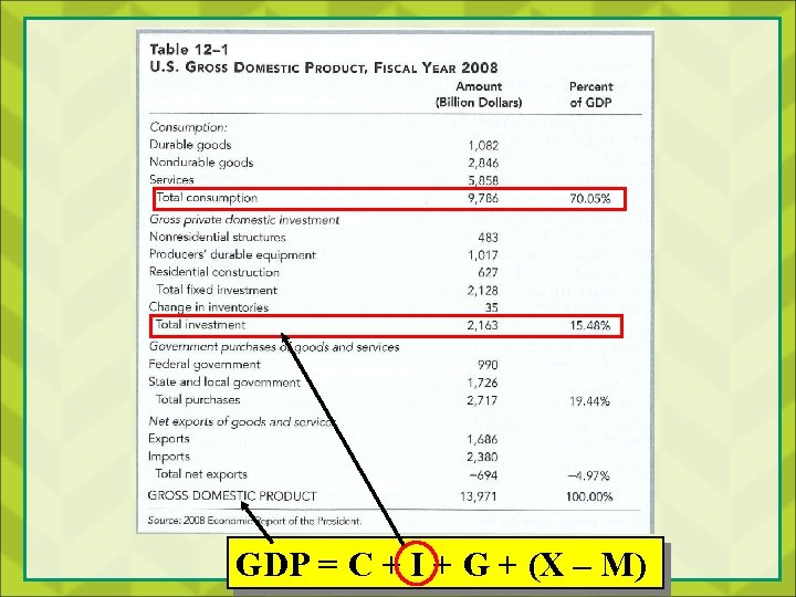
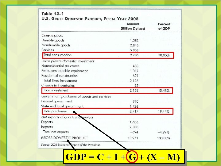
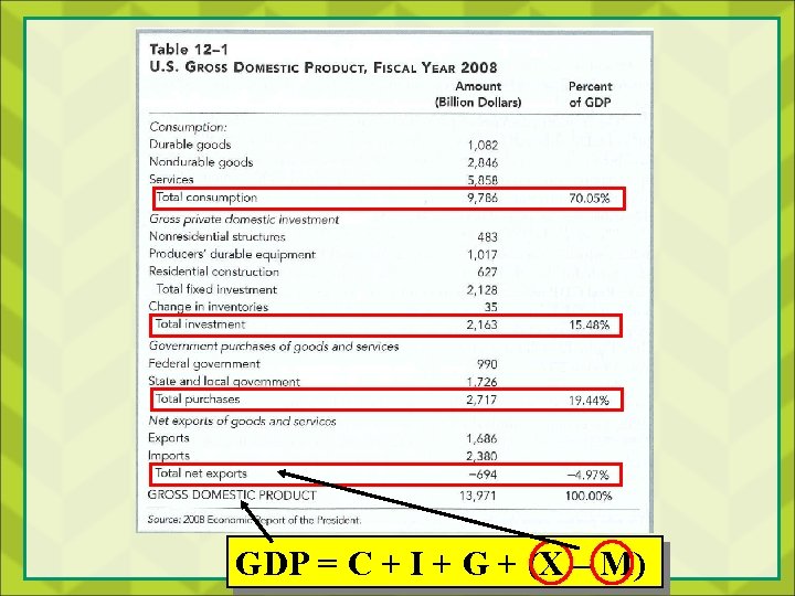
Measurement of Gross Domestic Product

GDP

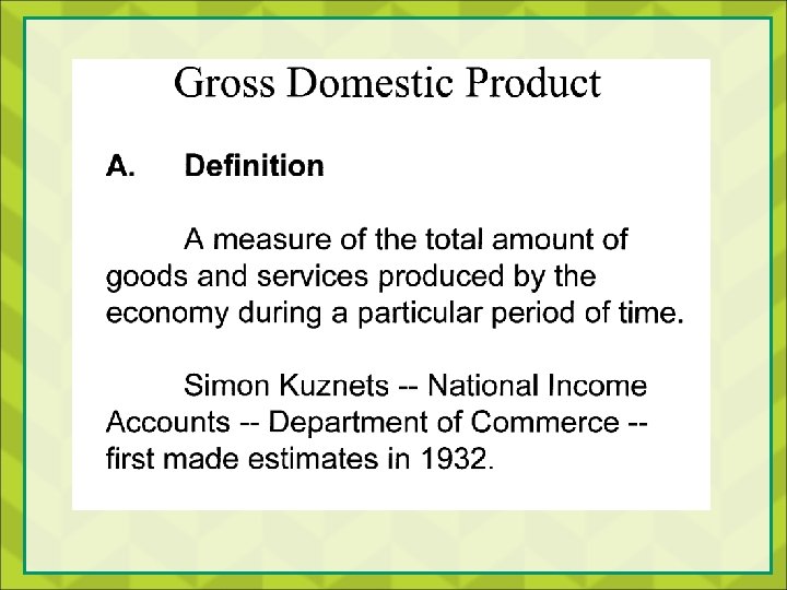
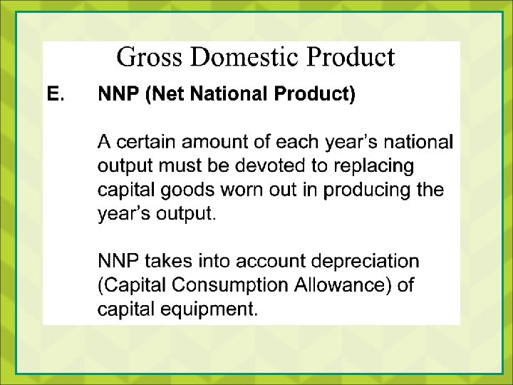
Gross Domestic Product B. Measurement Money – a common denominator ; add up the value of money in terms of the total output of goods and services during a certain time period, normally a year.

Everything below zero represents a recession Page 227

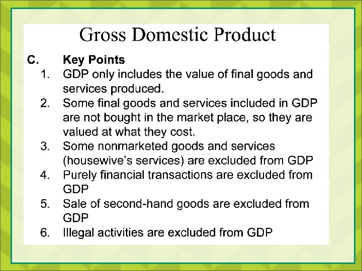
What’s in GDP? Focus is on new goods and services produced in current year

Types of consumer expenditures… Page 226

Types of investment expenditures… Page 226

Calculation of net exports… Page 226

Types of government Expenditures… Page 226

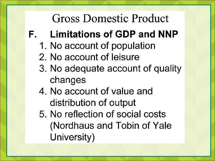
Items not included in GDP… Page 226

Understanding the Domestic Determinants of GDP C, I, G

Planned Consumption Function The slope of the consumption function is the marginal propensity to consume (MPC), or C÷ YD where YD represents disposable income. Autonomous or fixed consumption Page 228

Planned Consumption Function The consumption function in this graph can be expressed graphically as shown below. C = AC + MPC(DPI) Page 228

Planned Consumption Function Consumer expenditures would be $3, 600 if disposable income was equal to $3, 000. Consumers would be dis-saving by $600. C = $1, 500 +. 70($3, 000) = $3, 600 Page 228

Planned Consumption Function An increase in disposable income to $4, 000 would raise expenditures to $4, 300. Dis-saving would fall to $300. C = $1, 500 +. 70($4, 000) = $4, 300 Page 228

Planned Consumption Function An increase in disposable income to $5, 000 would raise expenditures to $5, 000. Dis-saving would fall to zero. C = $1, 500 +. 70($5, 000) = $5, 000 Page 228

Savings vs. Consumption We said that the slope of the consumption function was the marginal propensity to consume, or: MPC = C ÷ DPI Savings is defined as S = DPI – C And, therefore, the marginal propensity to save is MPS = 1. 0 – MPC Page 228 and 229

Planned Consumption Function A role for fiscal policy here: A cut in the tax rate increases consumption. An increase in the tax rate decreases consumption. Page 228

Planned Consumption Function A role for fiscal policy here: A cut in the tax rate increases consumption. An increase in the tax rate decreases consumption. Page 228

Shifts in Consumption Function • Changes in the level of income correspond to movements along the consumption function • Factors that can shift the consumption function: – Increase/decrease in wealth of nation’s household sector – Expectations of higher income in the near future

Planned Investment Function Level of autonomous investment spending I = AI – MIS(i) Page 233

Planned Investment Function The slope of the investment function is the marginal interest sensitivity of investment or: MIS = I÷ i I = AI – MIS(i) Page 233

Planned Investment Function Level of investment expenditures would be $250 at an interest rate of 9 percent if MIS = 25. I = $475 – 25(9. 0) Page 233

Planned Investment Function Should interest rates fall to 7% as a result of events in the money market, investment expenditures would increase from $250 to $300. I = $475 – 25(7. 0) Page 233

Shifts in Investment Function • Profit expectations • Prices of new investment goods • Technological change • Taxes

Effects of Profit Expectations An increase in profit expectations would shift the investment function to the right (e. g. , would cause businesses to expand their planned investment expenditures by $50 at the same interest rate). I = $525 – 25(7. 0) Page 234

Understanding Product Market Equilibrium

Aggregate Expenditures= C+I+G Consumption expenditures function: C = $1, 500+0. 70(DPI) Page 235

Aggregate Expenditures Consumption expenditures function: C = $1, 500+0. 70(DPI) Investment expenditures function: I = $475 – 25(i) Page 235

Aggregate Expenditures Consumption expenditures function: C = $1, 500+0. 70(DPI) Investment expenditures function: I = $475 – 25(i) Government expenditures function: G = $880 Page 235

Aggregate Expenditures (AE) Consumption expenditures function: C = $1, 500+0. 70(DPI) Investment expenditures function: I = $475 – 25(i) Government expenditures function: G = $880 If the interest rate (i) is equal to 7%, then AE = $1, 500 + 0. 70(DPI) + $475 – 25(7) +$880 = $2, 680 + 0. 70(DPI) Page 235

Aggregate Expenditures Aggregate expenditures equation: AE = $2, 680+0. 70(NI-Tax) Page 235

Aggregate Expenditures Aggregate expenditures equation: AE = $2, 680+0. 70(NI-Tax) where national output equals national income (NI) and Tax is based upon last year’s income (Tax = $400). Page 235

Aggregate Expenditures Aggregate expenditures equation: AE = $2, 680+0. 70(NI-Tax) where national output equals national income (NI) and Tax is based upon last year’s income (Tax = $400). If national income is $6, 000, then AE = $2, 680+0. 70($6, 000 - $400) = $6, 600 which represents the first line in Table 12. 4 Page 235

Aggregate Expenditures Aggregate expenditures equation: AE = $2, 680+0. 70(NI-Tax) where national output equals national income (NI) and Tax is based upon last year’s income (Tax = $400). If national income is $6, 000, then AE = $2, 680+0. 70($6, 000 - $400) = $6, 600 which represents the first line in Table 12. 4 Repeating this for other levels of income gives us the graph on page 236

Aggregate Expenditures Curve Total autonomous domestic spending… Page 236

Aggregate Expenditures Curve Point where spending equals output Y=C+I+G. This equilibrium assumes a given market interest rate and general price level. Note: below this equilibrium, AE>Y which should draw down unsold inventories and increase pressures to expand Y. Page 236

Deriving the Aggregate Demand Curve Aggregate demand curve Demand equals supply Corresponding price level Page 237

Aggregate Supply Curve: represents the nation’s output supplied to consumers, businesses, governments, foreign countries Three distinct ranges of the aggregate supply curve Page 238

Aggregate Supply Curve Maximum potential output in the short run: economy reaches capacity to supply goods and services in current period End of depression or Keynesian range: increases in demand supply unaccompanied by rising prices Page 238

Product Market Equilibrium YFE represents full employment output: economy’s max non-inflationary or natural rate of employment YE represents current or actual output (planned spending) YPOT represents potential or maximum output Page 238

Product Market Equilibrium : theoretical goal is to eliminate inflationary or recessionary gaps YE > YFE > YE Planned spending exceeds full employment output, causing higher inflationary pressures in economy. Planned spending less than full employment output, causing underutilization of economy’s resources. Page 238

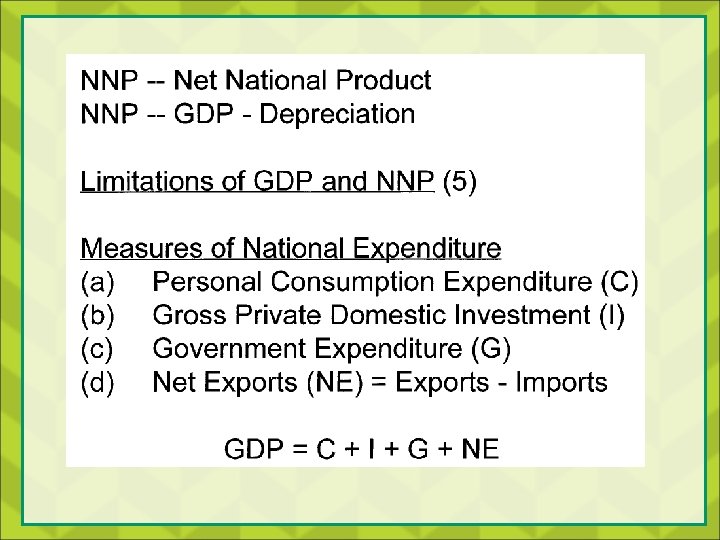
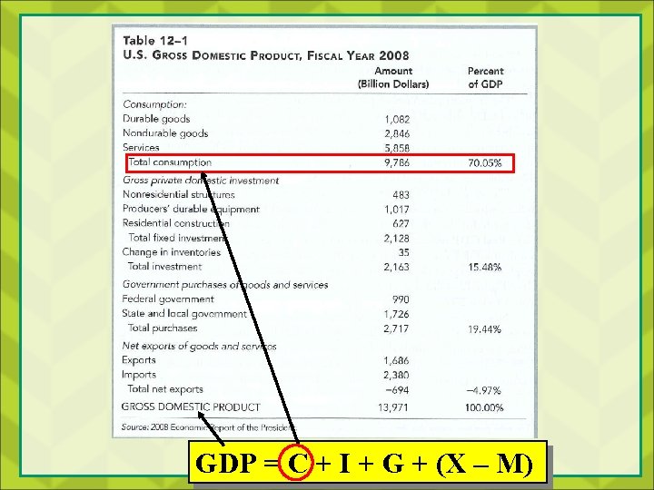
Summary ü GDP consists of C, I, G and (X-M) ü Focus is on new goods produced and services performed in the current year ü Consumption influenced by disposable income and wealth ü Investment influenced by interest rates and profit expectations ü Product market equilibrium occurs where aggregate demand equals aggregate supply ü Inflationary and recessionary gaps occur