Population Genetics Copyright The Mc GrawHill Companies Inc

Population Genetics Copyright © The Mc. Graw-Hill Companies, Inc. Permission required for reproduction or display.

Population genetics • Concerned with changes in genetic variation within a group of individuals over time • Want to know: – Extent of variation within population – Why variation exists – How variation changes over time • Study the gene pool – All alleles of every gene in a population

Population • Group of individuals of the same species that occupy the same region and can interbreed with one another • Local population (demes) – Smaller groups within population – Separated by moderate geographic barrier – More likely to interbreed Two local populations of douglas fir

Figure 24. 1 Populations • Dynamic – Size • Feast or famine – Geographic location • Migrate to new site with new environment – Consequences of changes in size and location • Changes in genetic composition

Polymorphism • “many forms” • Traits display variation within population • Ex. happy face spider – Differ in alleles that affect color and pattern • At the DNA level: – Multiple alleles for gene – Involves changes in DNA: deletion, duplication, single nucleotide change • SNP – most common – Monomorphism – single allele within population

Figure 24. 3 Polymorphism in humans • Human b-globin gene • Hb. A - normal gene • Hb. S - differs by SNP – Homozygous for Hb. S sickle cell anemia • Deletion – Loss of function allele

Two important frequency calculations • Allele frequency = (Number of copies of an allele in population) / (Total number of alleles for that gene in the population) • Genotype frequency = (Number of individuals with a particular genotype in a population) / (Total number of individuals in a population)

An example • 100 pea plants – 64 tall (TT) – 32 tall (Tt) – 4 dwarf (tt) • Allele frequency = number of copies of allele / total number of alleles – To calculate the frequency of ‘t’ • (32 + 8)/200 = 0. 2 or 20 % • What would be the frequency of ‘T’? • Genotype frequency = number of individuals with particular genotype / total number of individuals – To calculate the frequency of ‘tt’ • 4/100 = 0. 04 = 4% • Frequencies must always be less than or equal to 1 (100%)

Hardy Weinberg Equilibrium • Allele and genotype frequencies in a population are not changing over the course of many generations

Hardy-Weinberg Equation • Allows us to calculate allele and genotype frequencies • If gene is polymorphic and exists in two alleles, then p + q = 1 • p 2 + 2 pq + q 2 = 1 • p 2 = genotype frequency of AA • 2 pq = genotype frequency of Aa • q 2 = genotype frequency of aa

Applying the HW equation • Assume that gene exists as two different alleles: G and g. • If p = 0. 8, then what is the genotype frequency of gg?

Applying the HW equation • Assume that gene exists as two different alleles: G and g. • If p = 0. 8, then what is the genotype frequency of gg? • p = allele frequency of G • p + q = 1 so q = 0. 2 • q 2 = genotype frequency of gg = (0. 2)2 = 0. 04 = 4%

Figure 24. 4 Confirm with product rule

HW – predicting carriers • Allows us to determine the frequency of heterozygotes for recessive genetic diseases • Ex. Cystic fibrosis • Frequency of affected individuals (homozygous recessive) is 1 in 2500 • What is the frequency of heterozygous carriers?

HW – predicting carriers • • q 2 = 1/2500 q = √(1/2500) = 0. 02 p + q = 1 so p = 0. 98 Frequency of heterozygous carriers = 2 pq = 2(0. 02)(0. 98) = 0. 0392 = 3. 92%

Conditions for Hardy-Weinberg with regard to gene of interest • No new mutations: The gene of interest does not incur any new mutations • No genetic drift: The population is so large that allele frequencies do not change due to random sampling effects • No migration: Individuals do not travel between different populations • No natural selection: All of the genotypes have the same reproductive success • Random mating: With respect to the gene of interest, the members of the population mate with each other without regard to their phenotypes and genotypes

Figure 24. 5 Relationship between allele frequencies and genotype frequencies according to Hardy-Weinberg

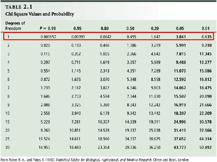
Use chi-square to determine if population exhibits Hardy-Weinberg equilibrium for gene • MN blood type • 200 people – 168 MM – 30 MN – 2 NN • First, calculate allele frequency of M and allele frequency of N • Then find expected MM, MN, and NN and solve chi-square equation

Chi square analysis • Allele frequency of M = (2(168)+30)/400 = 0. 915 = p • Allele frequency of N = (2(2)+30)/400 = 0. 085 = q

• Expected frequency of MM = p 2 = (0. 915)2 = 0. 837 – Expected number of MM individuals = (200 people)(0. 837) = 167 • Expected frequency of MN = 2 pq = 2(0. 915)(0. 085) = 0. 007 – Expected number of MN individuals = (200 people)(0. 007) = 1 • Expected frequency of NN = q 2 = (0. 085)2 = 0. 156 – Expected number of NN individuals = (200 people)(0. 156) = 31

Chi square analysis • Apply the ᵪ 2 formula • ∑((observed-expected)2/expected) • = ((168 -167)2/167) + ((30 -31)2/31) + ((2 -1)2/1) = 1. 04 • Degrees of freedom = n-1 – Gene exists in 2 alleles so n=2 so Dof. F = 1 – See chart – p > 0. 05 – Do not reject the Null hypothesis • Genes appear to be in HW equilibrium

• Genetic variation in natural population typically changes over many generations – Changes in gene pool

Mutations • Random events that occur spontaneously at a low rate or are caused by mutagens at a higher rate • Mutations can provide new alleles to a population but do not substantially alter allele frequencies

Mutations – an example • Mutation rate – probability that gene will be altered by a new mutation – 10 -5 to 10 -6 per generation • How much does mutation affect allele frequency? • Consider a mutation that converts A to a where the allele frequency of “A” = p and the allele frequency of “a” = q

Mutation – an exmple • Consider that Dq = mp (p decreases as A is converted to a) • Let’s assume: p = frequency of A = 80%; q = frequency of a = 20% • Assume m (rate of conversion of A to a) = 10 -5 • To calculate change in allele frequency – (1 -m)t = (pt/p 0) – pt = allele frequency of A at time t; p 0 = allele frequency of A at time 0; t = time; m = mutation rate

Mutations – an example • What would be the allele frequency of p after 1 generation? – (1 -10 -5)1 = pt/0. 8 – p 1 = 0. 799992 – q 1 = 0. 200008 • What would be the allele frequency of p after 1000 generations? – (1 -10 -5)1000 = pt/0. 8 – p 1000 = 0. 792 – q 1000 = 0. 208 • Notice that the change in allele frequency is very low.

Figure 24. 6 Genetic Drift • Changes in allele frequencies due to random fluctuations • Small sample size – Large fluctuations between generations – Allele eliminated or fixed at 100% over fewer generations • Large sample size – Random sampling has smaller effect

New allele fixation / elimination • Must first calculate the expected number of new mutations – Depends on mutation rate (μ) and population size (N) – 2 Nμ • Note: New mutation is more likely in a large population • Probability of fixation = 1/2 N • Probability of elimination = 1 - (1/2 N)

New allele fixation / elimination • Probability of fixation = 1/2 N • Probability of elimination = 1 - (1/2 N) • Large population – Greater likelihood for mutation – But, greater likelihood that new mutation will be eliminated from the population • Small population – Decreased likelihood for mutation – But, greater likelihood that new mutation will be fixed in the population

How long will fixation take? • ṫ = average # of generations to achieve fixation • ṫ = 4 N – Note: Allele fixation takes much longer in larger populations

Genetic Drift – Take home message • Operates in random manner with regard to allele frequency – Regardless of the type of allele • Deleterious, neutral, beneficial • Eventually leads to allele fixation or elimination • Occurs more quickly in smaller population

Changes in population size and genetic drift • Bottleneck effect – Decrease in population size because of events such as earthquake, drought, destruction of habitat • Elimination without regard to genetic composition • Founder effect – Migration of small group of individuals to new location • Small group may not have same genetic composition as parent population

Figure 24. 7 Bottleneck effect An example: Low genetic variation thought to be due to previous bottleneck

Founder effect • An example: – Old Order Amish in Lancaster County, PA – 1770: 3 couples immigrated to US – 1960: 800 individuals • Very high prevalence of recessive form of dwarfism • Thought that one of original ancestors carried recessive mutation or new mutation occurred early on

Migration • Between two different established populations – May alter allele frequencies • New population (after migration) = conglomerate • Change in allele frequency in conglomerate Dp. C = m(p. D-p. R) m = proportion of migrants that make up conglomerate p. D = allele frequency in donor population p. R = allele frequency in original recipient population

Migration – an example • A donor population has an “A” allele frequency of 0. 7. A recipient population has an “A” allele frequency of 0. 3. 20 people join the recipient population which originally had 80 members. What is the allele frequency in the conglomerate?

Migration – an example Dp. C = m(p. D-p. R) • m = 20/(20+80) • p. D = 0. 7 • p. R = 0. 3 Dp. C = 0. 2(0. 7 -0. 3) = 0. 08 p. C = allele frequency in conglomerate p. C = p. R + Dp. C = 0. 3 + 0. 08 = 0. 038

Migration • Often bidirectional flow • Tends to reduce differences in allele frequencies between neighboring populations

Natural selection • Conditions found in nature result in the selective survival and reproduction of individuals whose characteristics make them well adapted to their environment • Surviving individuals are more likely to reproduce and contribute offspring to the next generation

• Must consider Darwinian fitness – Relative likelihood that a phenotype will survive and contribute to the gene pool of the next generation – measure of reproductive superiority – Not same as physical fitness • Consider a gene with two alleles, A and a – The three genotypic classes can be assigned fitness values according to their reproductive potential Copyright ©The Mc. Graw-Hill Companies, Inc. Permission required for reproduction or display 24 -45

• Suppose the average reproductive success is – AA 5 offspring – Aa 4 offspring – aa 1 offspring • By convention, the gene with the highest reproductive ability is given fitness value of 1. 0 – The fitness values of the other genotypes are assigned relative to 1 • Fitness values are denoted by the variable W – Fitness of AA: WAA = 1. 0 – Fitness of Aa: WAa = 4/5 = 0. 8 – Fitness of aa: Waa = 1/5 = 0. 2 Copyright ©The Mc. Graw-Hill Companies, Inc. Permission required for reproduction or display 24 -46

• Differences in reproductive achievement could be due to the – 1. Fittest phenotype is more likely to survive – 2. Fittest phenotype is more likely to mate – 3. Fittest phenotype is more fertile Copyright ©The Mc. Graw-Hill Companies, Inc. Permission required for reproduction or display 24 -47

• Natural selection acts on phenotypes (which are derived from an individual’s genotype) • With regard to quantitative traits, there are four ways that natural selection may operate – 1. Directional selection • Favors the survival of one extreme phenotype that is better adapted to an environmental condition – 2. Stabilizing selection • Favors the survival of individuals with intermediate phenotypes – 3. Disruptive (or diversifying) selection • Favors the survival of two (or more) different phenotypes – 4. Balancing • Favors the maintenance of two or more alleles Copyright ©The Mc. Graw-Hill Companies, Inc. Permission required for reproduction or display 24 -48

• Directional Selection favor extreme phenotype – A gene exist in two alleles A and a – The three fitness values are • WAA = 1. 0 • WAa = 0. 8 • Waa = 0. 2 – In the next generation, the HW equilibrium will be modified in the following way by directional selection: • Frequency of AA: p 2 WAA • Frequency of Aa: 2 pq. WAa • Frequency of aa: q 2 Waa Copyright ©The Mc. Graw-Hill Companies, Inc. Permission required for reproduction or display 24 -49

– These three terms may not add up to 1. 0, as they would in the HW equilibrium – Instead, they sum to a value known as the mean fitness of the population • p 2 WAA + 2 pq. WAa + q 2 Waa = W – Divide both sides of the equation by the mean fitness of the population p 2 WAA W + 2 pq. WAa W + q 2 Waa =1 W – Now, calculate the expected genotype and allele frequencies after one generation of natural selection Copyright ©The Mc. Graw-Hill Companies, Inc. Permission required for reproduction or display 24 -50

– Frequency of AA genotype = p 2 WAA W – Frequency of Aa genotype = 2 pq. WAa W – Frequency of aa genotype = q 2 Waa W – Allele frequency of A: p. A = – Allele frequency of a: qa = p 2 WAA + W q 2 Waa W pq. WAa W + pq. WAa W Copyright ©The Mc. Graw-Hill Companies, Inc. Permission required for reproduction or display 24 -51

• Example: – Starting allele frequencies are A = 0. 5 and a = 0. 5 – Fitness values are 1. 0, 0. 8 and 0. 2 for genotypes AA, Aa and aa, respectively • p 2 WAA + 2 pq. WAa + q 2 Waa = W W = (0. 5)2(1) + 2(0. 5)(0. 8) + (0. 5)2(0. 2) = 0. 25 + 0. 4 + 0. 05 = 0. 7 – After one generation of selection: Copyright ©The Mc. Graw-Hill Companies, Inc. Permission required for reproduction or display 24 -52

– Frequency of AA genotype = p 2 WAA (0. 5)2(1) = = 0. 36 0. 7 W – Frequency of Aa genotype = 2 pq. WAa = 2(0. 5)(0. 8) 0. 7 W – Frequency of aa genotype = (0. 5)2(0. 2) = = 0. 07 0. 7 q 2 Waa W – Allele frequency of A: p. A = p 2 WAA = 0. 57 + W pq. WAa W = 0. 36 + 0. 57/2 = 0. 64 – Allele frequency of a: qa = q 2 Waa W + pq. WAa W = 0. 07 + 0. 57/2 = 0. 36 Copyright ©The Mc. Graw-Hill Companies, Inc. Permission required for reproduction or display 24 -53

• After one generation – f(A) has increased from 0. 5 to 0. 64 – f(a) has decreased from 0. 5 to 0. 36 – This is because the AA genotype has the highest fitness • Natural selection raises the mean fitness of the population – Assuming the individual fitness values are constant W = p 2 WAA + 2 pq. WAa + q 2 Waa = (0. 64)2(1) + 2(0. 64)(0. 36)(0. 8) + (0. 36)2(0. 2) = 0. 80 Copyright ©The Mc. Graw-Hill Companies, Inc. Permission required for reproduction or display 24 -54

General trend • increase A, decrease a, and increase the mean fitness of the population Copyright ©The Mc. Graw-Hill Companies, Inc. Permission required for reproduction or display 24 -55