Population Genetics Population Genetics Population genetics is concerned

Population Genetics

Population Genetics • Population genetics is concerned with the question of whether a particular allele or genotype will become more common or less common over time in a population, and Why. • Example: – Given that the CCR 5 -D 32 allele confers immunity to HIV, will it become more frequent in the human population over time?

Predicting Allele Frequencies Populations in Hardy-Weinberg equilibrium

Yule vs. Hardy • What are the characteristics of a population that is in equilibrium or another words, not evolving. • Yule thought that allele frequencies had to be 0. 5 and 0. 5. for a population to be in equilibrium. • Hardy proved him wrong by developing the Hardy-Weinburg equation.

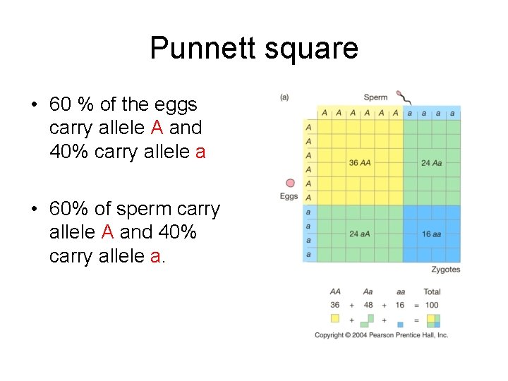
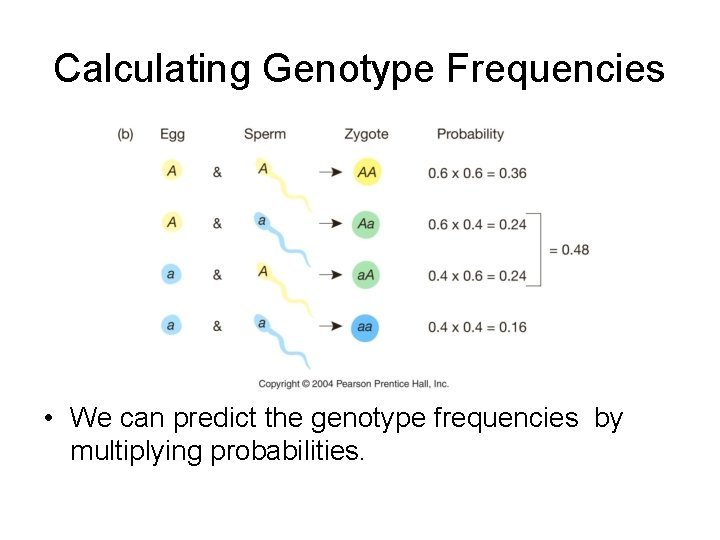
Punnett square • 60 % of the eggs carry allele A and 40% carry allele a • 60% of sperm carry allele A and 40% carry allele a.

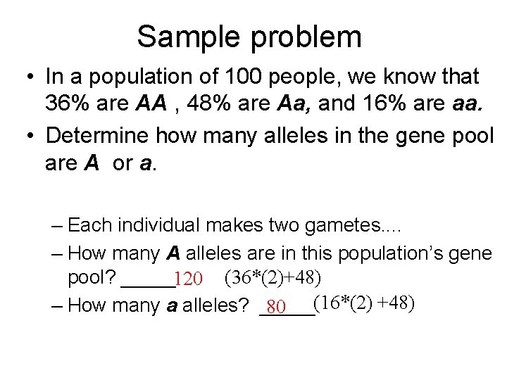
Sample problem • In a population of 100 people, we know that 36% are AA , 48% are Aa, and 16% are aa. • Determine how many alleles in the gene pool are A or a. – Each individual makes two gametes. . – How many A alleles are in this population’s gene pool? _____120 (36*(2)+48) (16*(2) +48) – How many a alleles? _____ 80

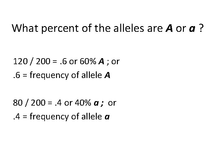
What percent of the alleles are A or a ? 120 / 200 =. 6 or 60% A ; or. 6 = frequency of allele A 80 / 200 =. 4 or 40% a ; or. 4 = frequency of allele a

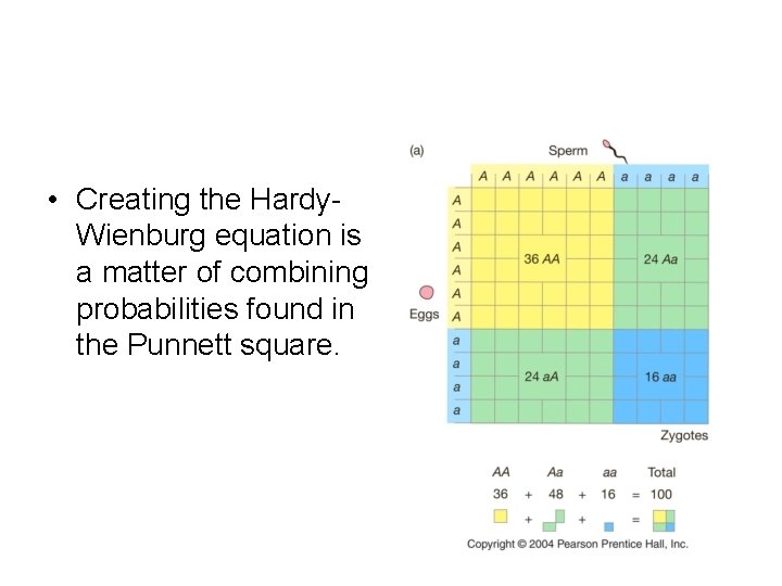
• Creating the Hardy. Wienburg equation is a matter of combining probabilities found in the Punnett square.

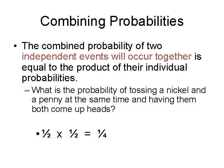
Combining Probabilities • The combined probability of two independent events will occur together is equal to the product of their individual probabilities. – What is the probability of tossing a nickel and a penny at the same time and having them both come up heads? • ½ x ½ = ¼

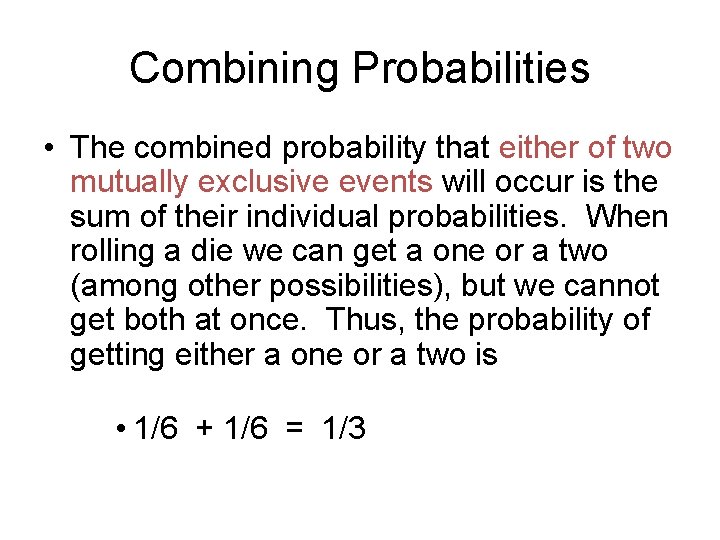
Combining Probabilities • The combined probability that either of two mutually exclusive events will occur is the sum of their individual probabilities. When rolling a die we can get a one or a two (among other possibilities), but we cannot get both at once. Thus, the probability of getting either a one or a two is • 1/6 + 1/6 = 1/3

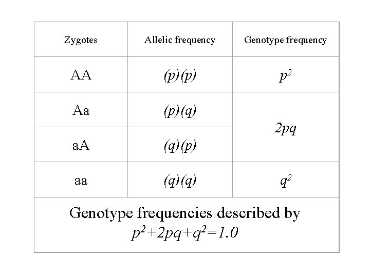
Calculating Genotype Frequencies • We can predict the genotype frequencies by multiplying probabilities.

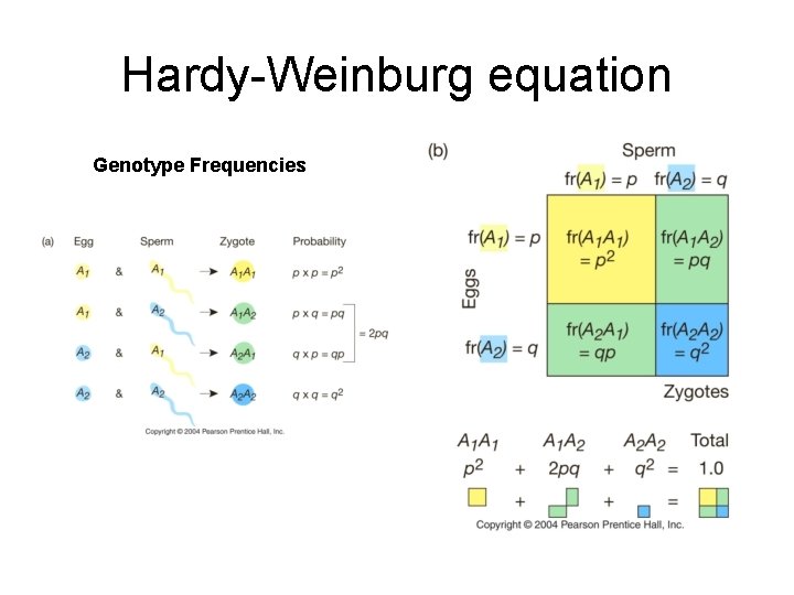
Hardy-Weinburg equation Genotype Frequencies

Zygotes Allelic frequency Genotype frequency AA (p)(p) p 2 Aa (p)(q) 2 pq a. A (q)(p) aa (q)(q) q 2 Genotype frequencies described by 2=1. 0 p 2+2 pq+q

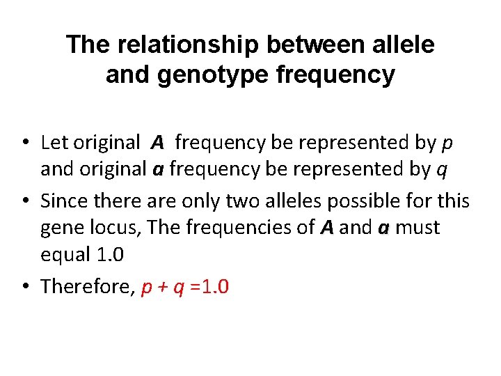
The relationship between allele and genotype frequency • Let original A frequency be represented by p and original a frequency be represented by q • Since there are only two alleles possible for this gene locus, The frequencies of A and a must equal 1. 0 • Therefore, p + q =1. 0

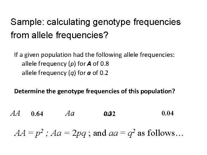
Sample: calculating genotype frequencies from allele frequencies? If a given population had the following allele frequencies: allele frequency (p) for A of 0. 8 allele frequency (q) for a of 0. 2 Determine the genotype frequencies of this population? AA Aa 0. 64 aa 0. 32 0. 04 2 ; Aa = 2 pq ; and aa = q 2 as follows… AA = p AA aa

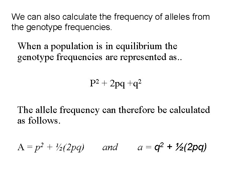
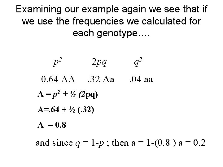
We can also calculate the frequency of alleles from the genotype frequencies. When a population is in equilibrium the genotype frequencies are represented as. . P 2 + 2 pq +q 2 The allele frequency can therefore be calculated as follows. A = p 2 + ½(2 pq) and a = q 2 + ½(2 pq)

Examining our example again we see that if we use the frequencies we calculated for each genotype…. p 2 2 pq q 2 0. 64 AA . 32 Aa . 04 aa A = p 2 + ½ (2 pq) A=. 64 + ½ (. 32) A = 0. 8 and since q = 1 -p ; then a = 1 -(0. 8 ) a = 0. 2

These rules hold as long as a population is in equilibrium. Hardy Weinberg Equilibrium describes the conclusions and assumptions that must be present to consider a population in equilibrium.

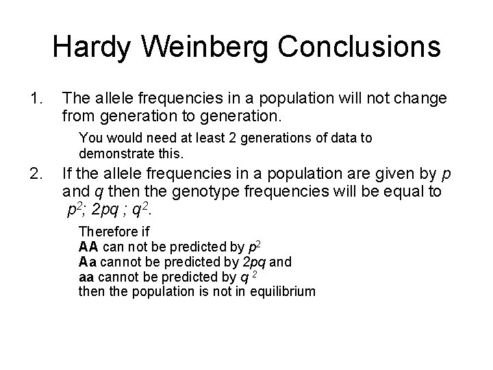
Hardy Weinberg Conclusions 1. The allele frequencies in a population will not change from generation to generation. You would need at least 2 generations of data to demonstrate this. 2. If the allele frequencies in a population are given by p and q then the genotype frequencies will be equal to p 2; 2 pq ; q 2. Therefore if AA can not be predicted by p 2 Aa cannot be predicted by 2 pq and aa cannot be predicted by q 2 then the population is not in equilibrium

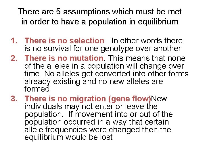
There are 5 assumptions which must be met in order to have a population in equilibrium 1. There is no selection. In other words there is no survival for one genotype over another 2. There is no mutation. This means that none of the alleles in a population will change over time. No alleles get converted into other forms already existing and no new alleles are formed 3. There is no migration (gene flow)New individuals may not enter or leave the population. If movement into or out of the population occurred in a way that certain allele frequencies were changed then the equilibrium would be lost

Exceptions to Hardy Weinberg cont. 4. There are no chance events (genetic drift) This can only occur if the population is sufficiently large to ensure that the chance of an offspring getting one allele or the other is purely random. When populations are small the principle of genetic drift enters and the equilibrium is not established or will be lost as population size dwindles due to the effects of some outside influence 5. There is no sexual selection or mate choice Who mates with whom must be totally random with no preferential selection involved.

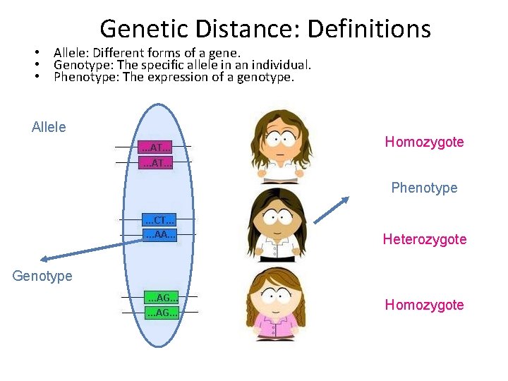
Genetic Distance: Definitions • Allele: Different forms of a gene. • Genotype: The specific allele in an individual. • Phenotype: The expression of a genotype. Allele Homozygote Phenotype Heterozygote Genotype Homozygote

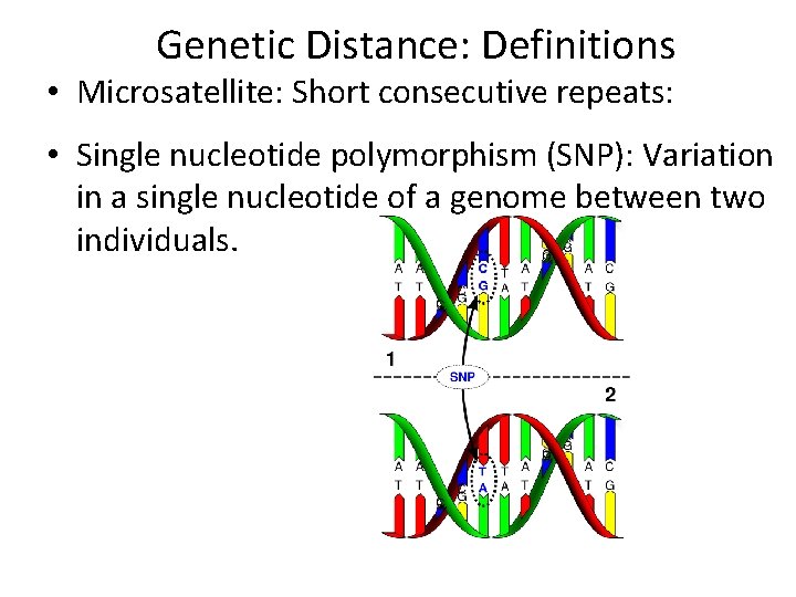
Genetic Distance: Definitions • Microsatellite: Short consecutive repeats: • Single nucleotide polymorphism (SNP): Variation in a single nucleotide of a genome between two individuals.

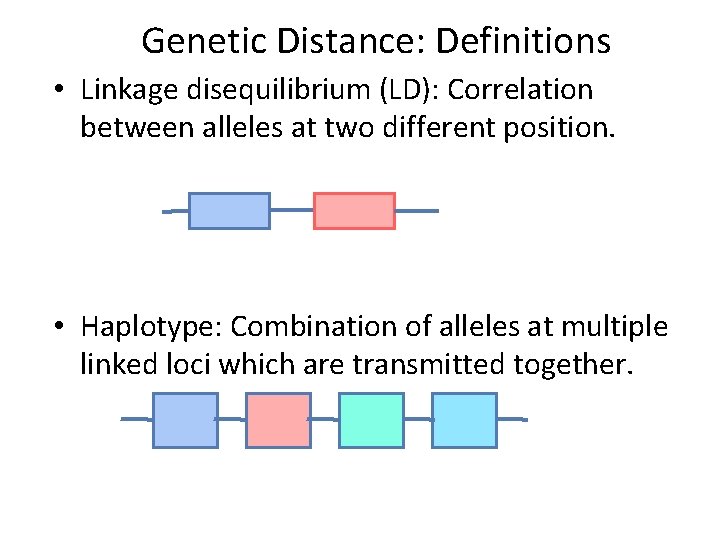
Genetic Distance: Definitions • Linkage disequilibrium (LD): Correlation between alleles at two different position. • Haplotype: Combination of alleles at multiple linked loci which are transmitted together.

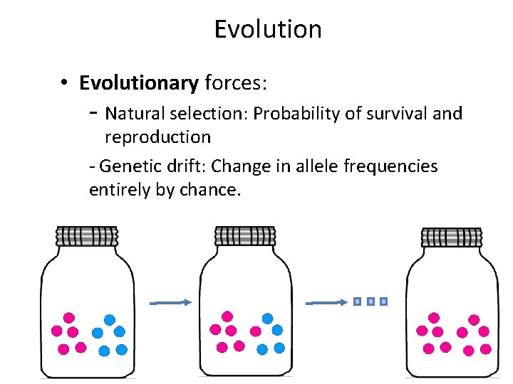
Evolution • Evolutionary forces: - Natural selection: Probability of survival and reproduction - Genetic drift: Change in allele frequencies entirely by chance.

Selection vs Drift The two forces that determine the fate of alleles in a population • Drift – Change in allele frequencies due to sampling – a ‘stochastic’ process – Neutral variation is subject to drift • Selection – Change in allele frequencies due to function – ‘deterministic’ – Functional variation may be subject to selection (more later)

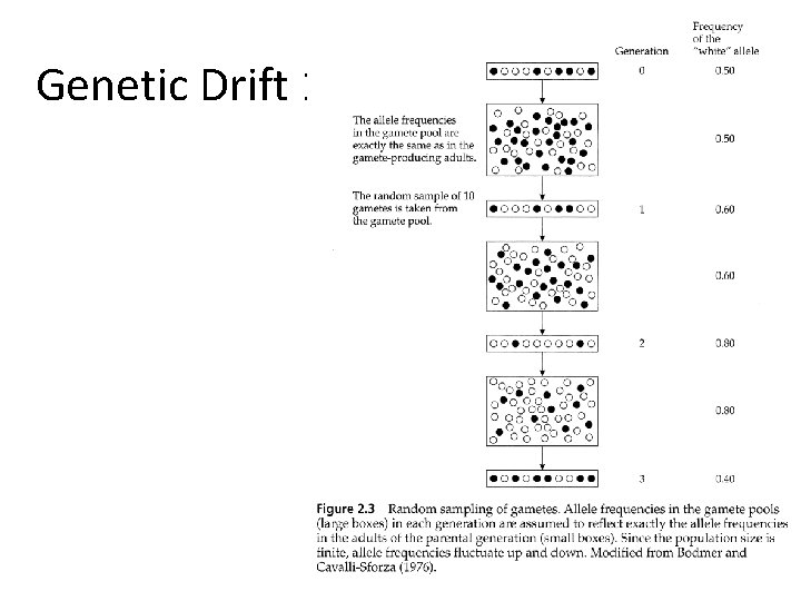
Genetic Drift 1

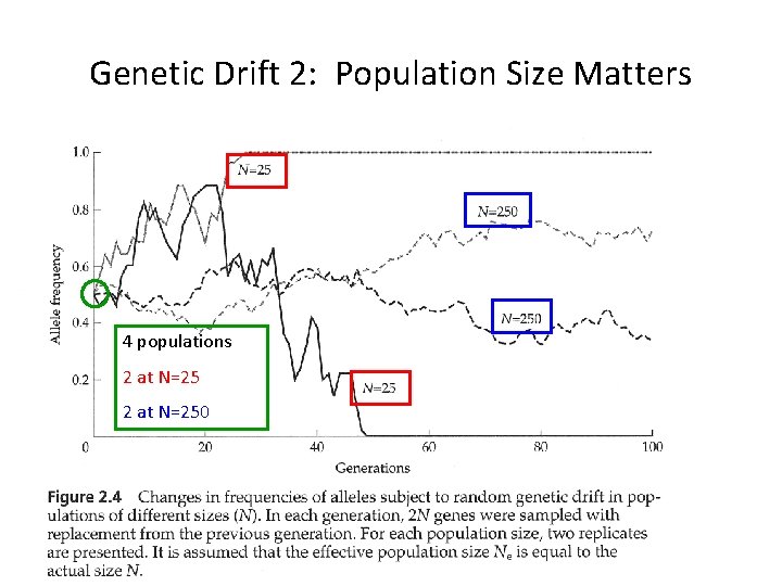
Genetic Drift 2: Population Size Matters 4 populations 2 at N=250

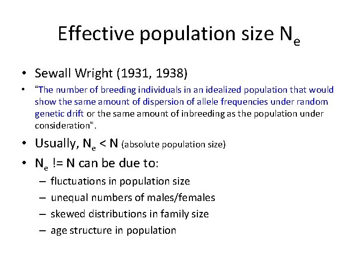
Effective population size Ne • Sewall Wright (1931, 1938) • “The number of breeding individuals in an idealized population that would show the same amount of dispersion of allele frequencies under random genetic drift or the same amount of inbreeding as the population under consideration". • Usually, Ne < N (absolute population size) • Ne != N can be due to: – – fluctuations in population size unequal numbers of males/females skewed distributions in family size age structure in population

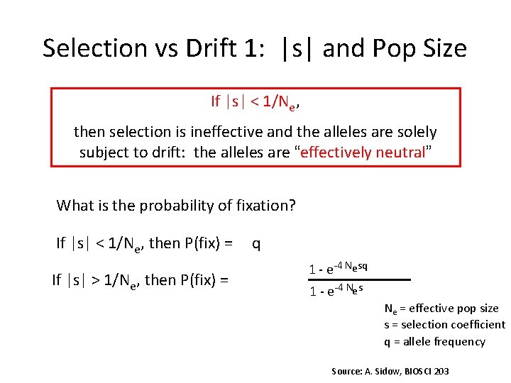
Selection vs Drift 1: |s| and Pop Size If |s| < 1/Ne, then selection is ineffective and the alleles are solely subject to drift: the alleles are “effectively neutral” What is the probability of fixation? If |s| < 1/Ne, then P(fix) = If |s| > 1/Ne, then P(fix) = q 1 - e-4 Ne s Ne = effective pop size s = selection coefficient q = allele frequency Source: A. Sidow, BIOSCI 203

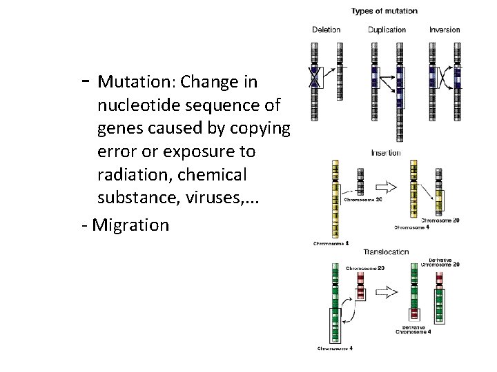
- Mutation: Change in nucleotide sequence of genes caused by copying error or exposure to radiation, chemical substance, viruses, . . . - Migration

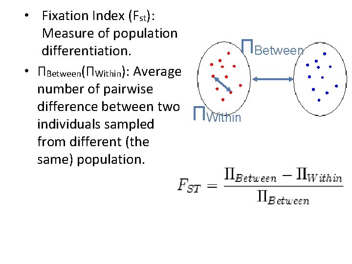
• Fixation Index (Fst): Measure of population differentiation. • ΠBetween(ΠWithin): Average number of pairwise difference between two individuals sampled from different (the same) population. ΠBetween ΠWithin

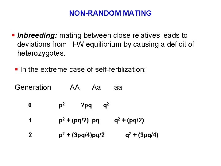
NON-RANDOM MATING § Inbreeding: mating between close relatives leads to deviations from H-W equilibrium by causing a deficit of heterozygotes. § In the extreme case of self-fertilization: Generation AA Aa 2 pq aa 0 p 2 q 2 1 p 2 + (pq/2) pq 2 p 2 + (3 pq/4)pq/2 q 2 + (pq/2) q 2 + (3 pq/4)

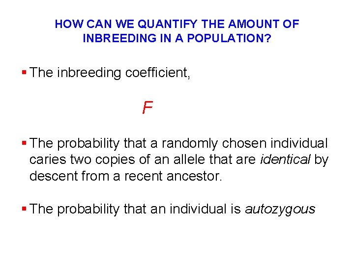
HOW CAN WE QUANTIFY THE AMOUNT OF INBREEDING IN A POPULATION? § The inbreeding coefficient, F § The probability that a randomly chosen individual caries two copies of an allele that are identical by descent from a recent ancestor. § The probability that an individual is autozygous

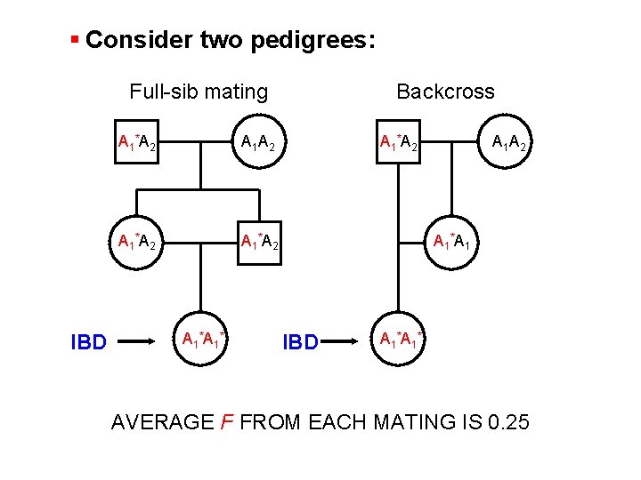
§ Consider two pedigrees: Full-sib mating IBD A 1 *A 2 A 1 *A 1 * Backcross A 1 *A 2 A 1 *A 1 IBD A 1 * AVERAGE F FROM EACH MATING IS 0. 25

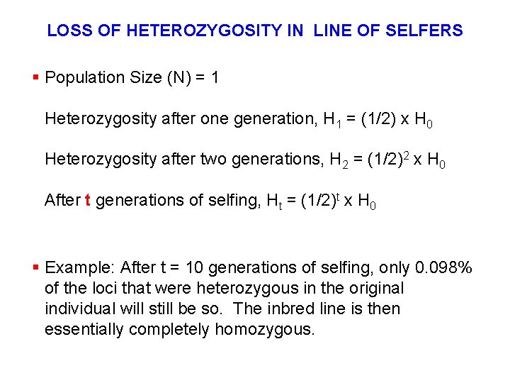
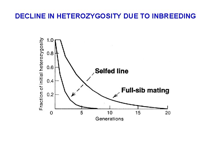
LOSS OF HETEROZYGOSITY IN LINE OF SELFERS § Population Size (N) = 1 Heterozygosity after one generation, H 1 = (1/2) x H 0 Heterozygosity after two generations, H 2 = (1/2)2 x H 0 After t generations of selfing, Ht = (1/2)t x H 0 § Example: After t = 10 generations of selfing, only 0. 098% of the loci that were heterozygous in the original individual will still be so. The inbred line is then essentially completely homozygous.

DECLINE IN HETEROZYGOSITY DUE TO INBREEDING

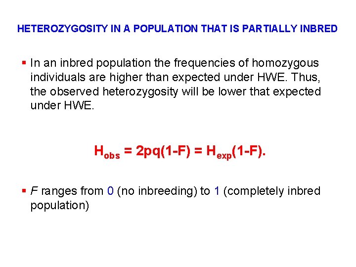
HETEROZYGOSITY IN A POPULATION THAT IS PARTIALLY INBRED § In an inbred population the frequencies of homozygous individuals are higher than expected under HWE. Thus, the observed heterozygosity will be lower that expected under HWE. Hobs = 2 pq(1 -F) = Hexp(1 -F). § F ranges from 0 (no inbreeding) to 1 (completely inbred population)

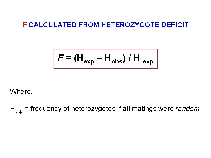
F CALCULATED FROM HETEROZYGOTE DEFICIT F = (Hexp – Hobs) / H exp Where, Hexp = frequency of heterozygotes if all matings were random

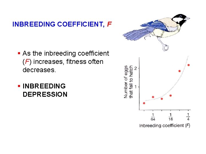
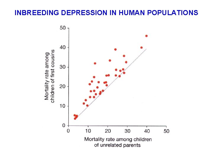
INBREEDING COEFFICIENT, F § As the inbreeding coefficient (F) increases, fitness often decreases. § INBREEDING DEPRESSION

INBREEDING DEPRESSION IN HUMAN POPULATIONS

INBREEDING VERSUS RANDOM GENETIC DRIFT § Inbreeding is caused by non-random mating and leads to changes in genotype frequencies but not allele frequencies. § Random genetic drift occurs in finite populations, even with completely random mating, and leads to changes in both genotype and allele frequencies. § Both processes cause a decline in heterozygosity.

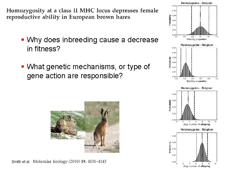
§ Why does inbreeding cause a decrease in fitness? § What genetic mechanisms, or type of gene action are responsible? Smith et al.

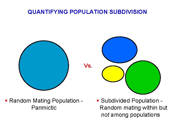
QUANTIFYING POPULATION SUBDIVISION Vs. § Random Mating Population Panmictic § Subdivided Population Random mating within but not among populations

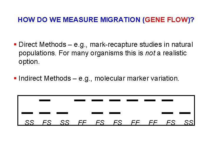
HOW DO WE MEASURE MIGRATION (GENE FLOW)? § Direct Methods – e. g. , mark-recapture studies in natural populations. For many organisms this is not a realistic option. § Indirect Methods – e. g. , molecular marker variation. SS FS SS FF FS FS FF FF FS SS

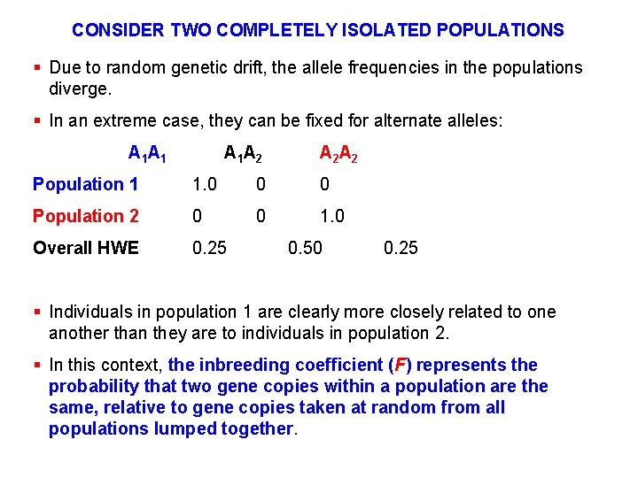
CONSIDER TWO COMPLETELY ISOLATED POPULATIONS § Due to random genetic drift, the allele frequencies in the populations diverge. § In an extreme case, they can be fixed for alternate alleles: A 1 A 1 A 2 A 2 Population 1 1. 0 0 0 Population 2 0 0 1. 0 Overall HWE 0. 25 0. 50 0. 25 § Individuals in population 1 are clearly more closely related to one another than they are to individuals in population 2. § In this context, the inbreeding coefficient (F) represents the probability that two gene copies within a population are the same, relative to gene copies taken at random from all populations lumped together.

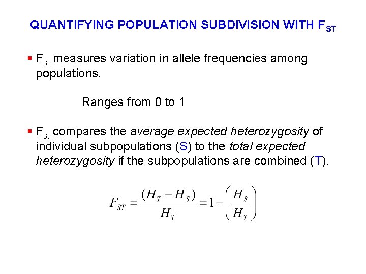
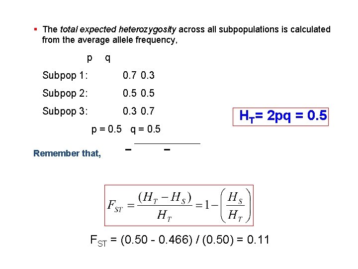
QUANTIFYING POPULATION SUBDIVISION WITH FST § Fst measures variation in allele frequencies among populations. Ranges from 0 to 1 § Fst compares the average expected heterozygosity of individual subpopulations (S) to the total expected heterozygosity if the subpopulations are combined (T).

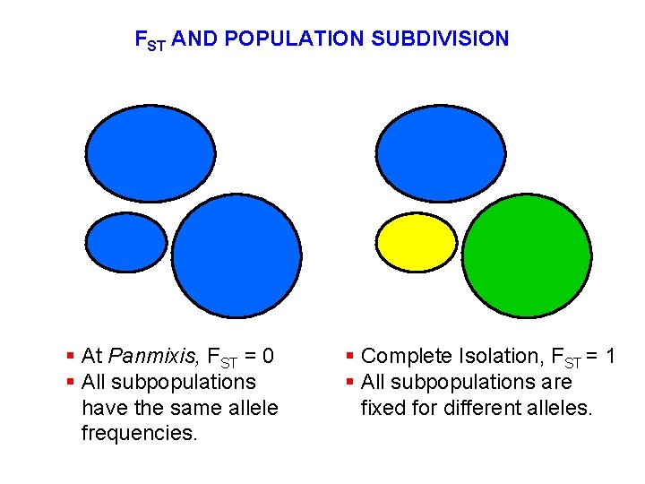
FST AND POPULATION SUBDIVISION § At Panmixis, FST = 0 § All subpopulations have the same allele frequencies. § Complete Isolation, FST = 1 § All subpopulations are fixed for different alleles.

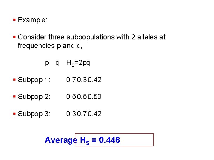
§ Example: § Consider three subpopulations with 2 alleles at frequencies p and q, p q HS=2 pq § Subpop 1: 0. 7 0. 3 0. 42 § Subpop 2: 0. 50 § Subpop 3: 0. 3 0. 7 0. 42 Average HS = 0. 446

§ The total expected heterozygosity across all subpopulations is calculated from the average allele frequency, p q Subpop 1: 0. 7 0. 3 Subpop 2: 0. 5 Subpop 3: 0. 3 0. 7 p = 0. 5 q = 0. 5 HT= 2 pq = 0. 5 Remember that, FST = (0. 50 - 0. 466) / (0. 50) = 0. 11

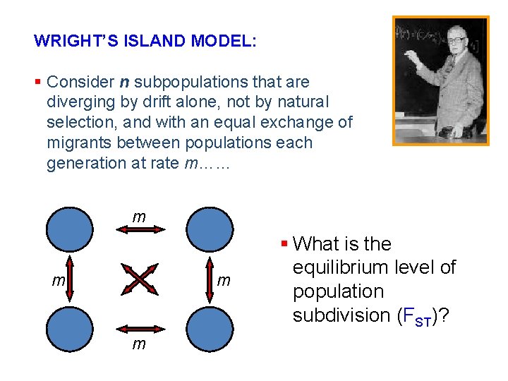
WRIGHT’S ISLAND MODEL: § Consider n subpopulations that are diverging by drift alone, not by natural selection, and with an equal exchange of migrants between populations each generation at rate m…… m m § What is the equilibrium level of population subdivision (FST)?

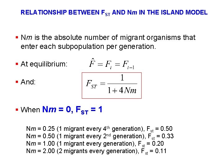
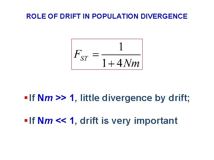
RELATIONSHIP BETWEEN FST AND Nm IN THE ISLAND MODEL § Nm is the absolute number of migrant organisms that enter each subpopulation per generation. § At equilibrium: § And: § When Nm = 0, FST = 1 Nm = 0. 25 (1 migrant every 4 th generation), Fst = 0. 50 Nm = 0. 50 (1 migrant every 2 nd generation), Fst = 0. 33 Nm = 1. 00 (1 migrant every generation), Fst = 0. 20 Nm = 2. 00 (2 migrants every generation), Fst = 0. 11

ROLE OF DRIFT IN POPULATION DIVERGENCE § If Nm >> 1, little divergence by drift; § If Nm << 1, drift is very important

• Find Genes which are candidates to have been under selection: Very low and very high Fst distance. Compare expected and observed values of Fst.

Detection of Selection in Humans with SNPs Large-scale SNP-survey looked at: 106 Genes in an average of 57 human individuals 60, 410 base pairs of noncoding sequence (UTRs, introns, some promoters) 135, 823 base pairs of coding sequence Some salient points: • Because survey is snapshot of current frequencies, evidence for selection or drift is indirect • This is about bulk properties, not about individual genes

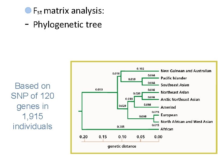
- Fst matrix analysis: Phylogenetic tree Based on SNP of 120 genes in 1, 915 individuals

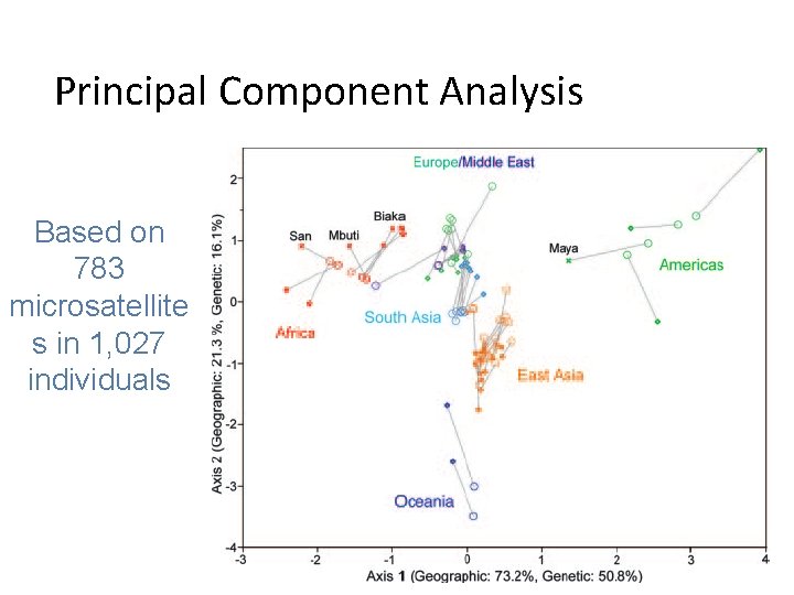
Principal Component Analysis Based on 783 microsatellite s in 1, 027 individuals

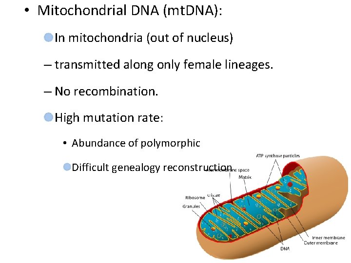
• Mitochondrial DNA (mt. DNA): In mitochondria (out of nucleus) – transmitted along only female lineages. – No recombination. High mutation rate: • Abundance of polymorphic Difficult genealogy reconstruction