Phenotypic factor analysis Conor Dolan Mike Neale Michel

Phenotypic factor analysis Conor Dolan, Mike Neale, & Michel Nivard

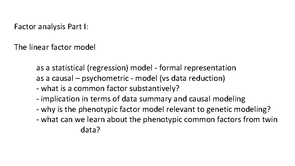
Factor analysis Part I: The linear factor model as a statistical (regression) model - formal representation as a causal – psychometric - model (vs data reduction) - what is a common factor substantively? - implication in terms of data summary and causal modeling - why is the phenotypic factor model relevant to genetic modeling? - what can we learn about the phenotypic common factors from twin data?

If you understand linear regression, you understand a key ingredient of the linear factor model (as a statistical model). If you understand logistic linear regression, you understand a key ingredient of the ordinal factor model (as a statistical model).

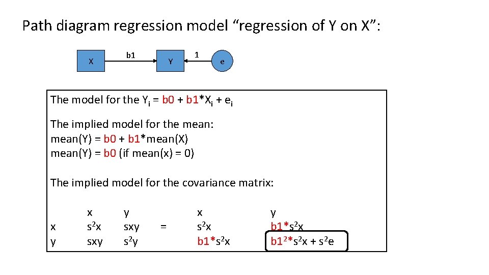
Path diagram regression model “regression of Y on X”: X b 1 Y 1 e The model for the Yi = b 0 + b 1*Xi + ei The implied model for the mean: mean(Y) = b 0 + b 1*mean(X) mean(Y) = b 0 (if mean(x) = 0) The implied model for the covariance matrix: x y x s 2 x sxy y sxy s 2 y = x s 2 x b 1*s 2 x y b 1*s 2 x b 12*s 2 x + s 2 e

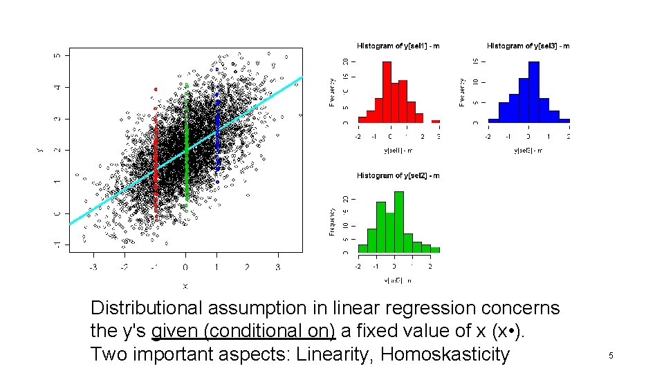
Distributional assumption in linear regression concerns the y's given (conditional on) a fixed value of x (x • ). Two important aspects: Linearity, Homoskasticity 5

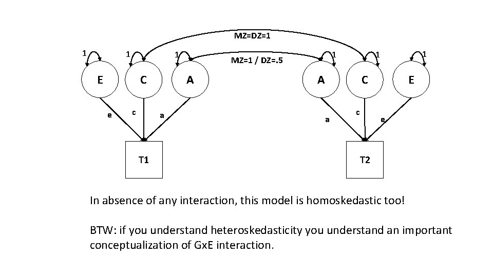
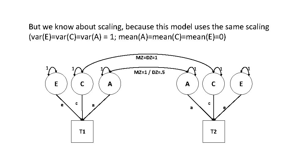
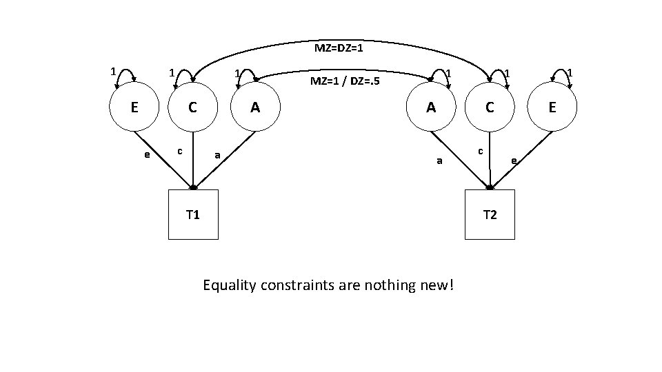
MZ=DZ=1 1 E A C e c a T 1 1 MZ=1 / DZ=. 5 1 1 A E C a c e T 2 In absence of any interaction, this model is homoskedastic too! BTW: if you understand heteroskedasticity you understand an important conceptualization of Gx. E interaction.

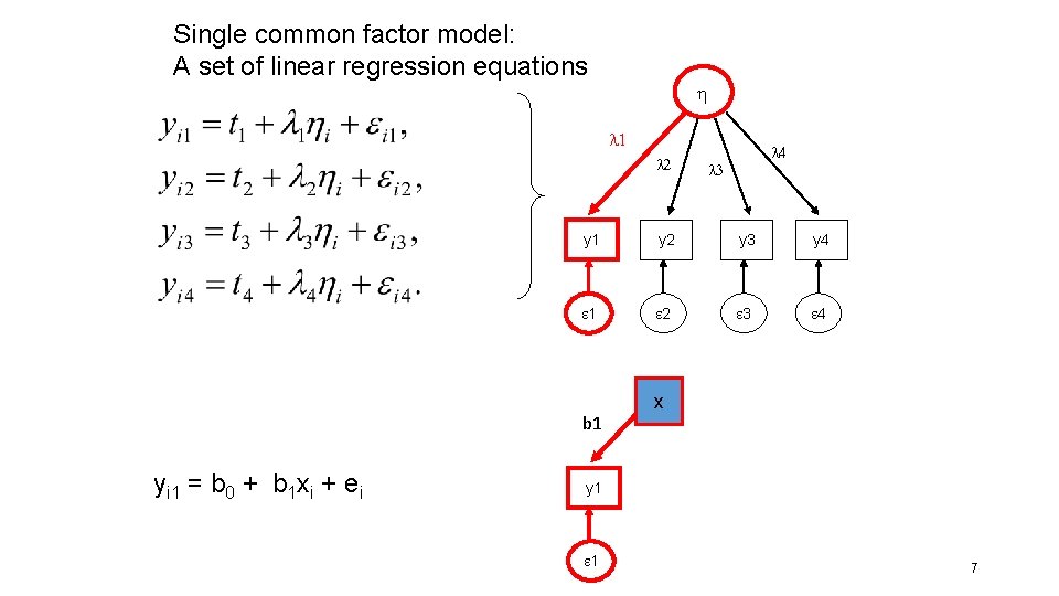
Single common factor model: A set of linear regression equations l 1 l 2 l 3 y 1 y 2 y 3 y 4 1 2 3 4 b 1 yi 1 = b 0 + b 1 xi + ei l 4 x y 1 1 7

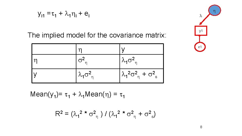
yi 1 =t 1 + l 1 i + ei l The implied model for the covariance matrix: y s 2 l 1 s 2 y l 1 s 2 l 1 2 s 2 + s 2 y 1 1 Mean(y 1)= t 1 + l 1 Mean( ) = t 1 R 2 = (l 12 * s 2 ) / (l 12 * s 2 + s 2 ) 8

But what is the point if the common factor (the independent variable, ) is not observed? 9

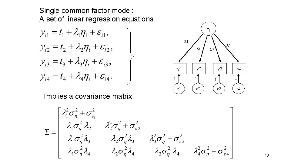
Single common factor model: A set of linear regression equations l 1 l 2 y 1 1 l 3 y 2 1 1 l 4 2 y 3 y 4 1 1 3 4 Implies a covariance matrix: 10

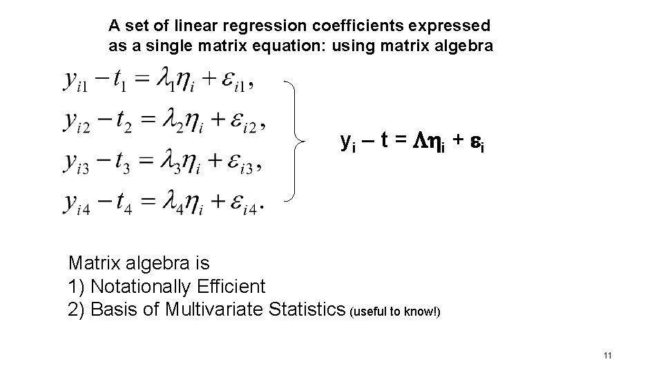
A set of linear regression coefficients expressed as a single matrix equation: using matrix algebra yi – t = i + i Matrix algebra is 1) Notationally Efficient 2) Basis of Multivariate Statistics (useful to know!) 11

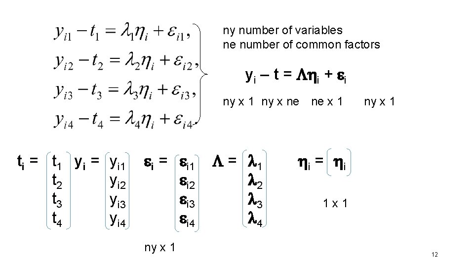
ny number of variables ne number of common factors yi – t = i + i ny x 1 ny x ne ne x 1 ti = t 1 y i = t 2 t 3 t 4 yi 1 yi 2 yi 3 yi 4 i = i 1 i 2 i 3 i 4 ny x 1 = l 1 l 2 l 3 l 4 ny x 1 i = i 1 x 1 12

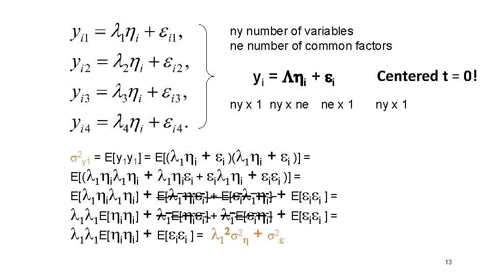
ny number of variables ne number of common factors yi = i + i ny x 1 ny x ne ne x 1 Centered t = 0! ny x 1 s 2 y 1 = E[y 1 y 1] = E[(l 1 i + i )] = E[(l 1 i + l 1 i i + il 1 i + i i )] = E[l 1 i] + E[l 1 i i] + E[ il 1 i] + E[ i i ] = l 1 l 1 E[ i i] + E[ i i ] = l 12 s 2 + s 2 13

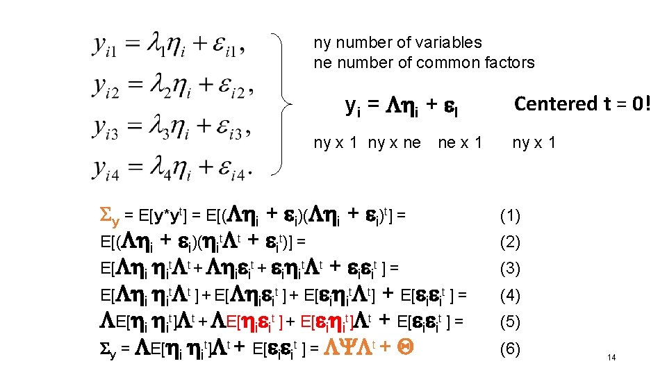
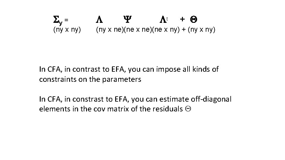
ny number of variables ne number of common factors yi = i + I ny x 1 ny x ne ne x 1 Sy = E[y*yt] = E[( i + i)t] = E[( i + i)( it t + it)] = E[ i it t + i it + i it ] = E[ i it t ] + E[ i it t] + E[ i it ] = E[ i it] t + E[ i it ] + E[ i it] t + E[ i it ] = Sy = E[ i it] t + E[ i it ] = Y t + Q Centered t = 0! ny x 1 (1) (2) (3) (4) (5) (6) 14

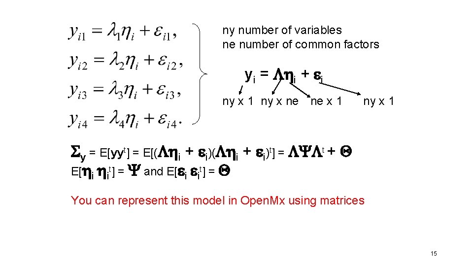
ny number of variables ne number of common factors yi = i + i ny x 1 ny x ne ne x 1 ny x 1 Sy = E[yyt] = E[( i + i)t] = Y t + Q E[ i it] = Y and E[ i it] = Q You can represent this model in Open. Mx using matrices 15

So what? What is the use?

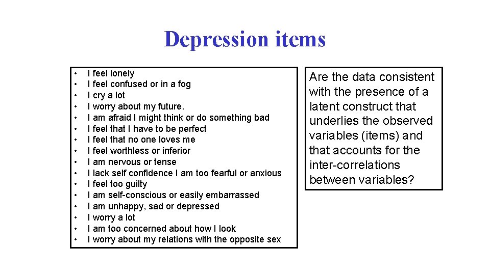
Depression items • • • • I feel lonely I feel confused or in a fog I cry a lot I worry about my future. I am afraid I might think or do something bad I feel that I have to be perfect I feel that no one loves me I feel worthless or inferior I am nervous or tense I lack self confidence I am too fearful or anxious I feel too guilty I am self-conscious or easily embarrassed I am unhappy, sad or depressed I worry a lot I am too concerned about how I look I worry about my relations with the opposite sex Are the data consistent with the presence of a latent construct that underlies the observed variables (items) and that accounts for the inter-correlations between variables?

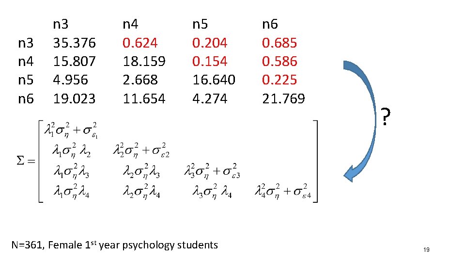
The use is to test the hypothesis that the linear relations among my 4 indicators of neuroticism, as expressed in the correlation or covariance matrix, are consistent with the presence of a single common influence, the latent variable “neuroticism”.

n 3 n 4 n 5 n 6 n 3 35. 376 15. 807 4. 956 19. 023 n 4 0. 624 18. 159 2. 668 11. 654 n 5 0. 204 0. 154 16. 640 4. 274 N=361, Female 1 st year psychology students n 6 0. 685 0. 586 0. 225 21. 769 ? 19

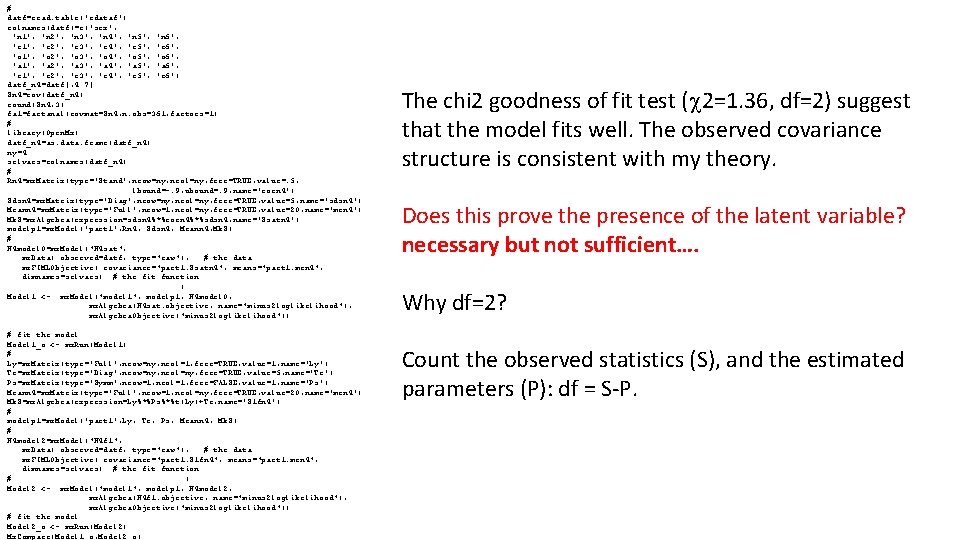
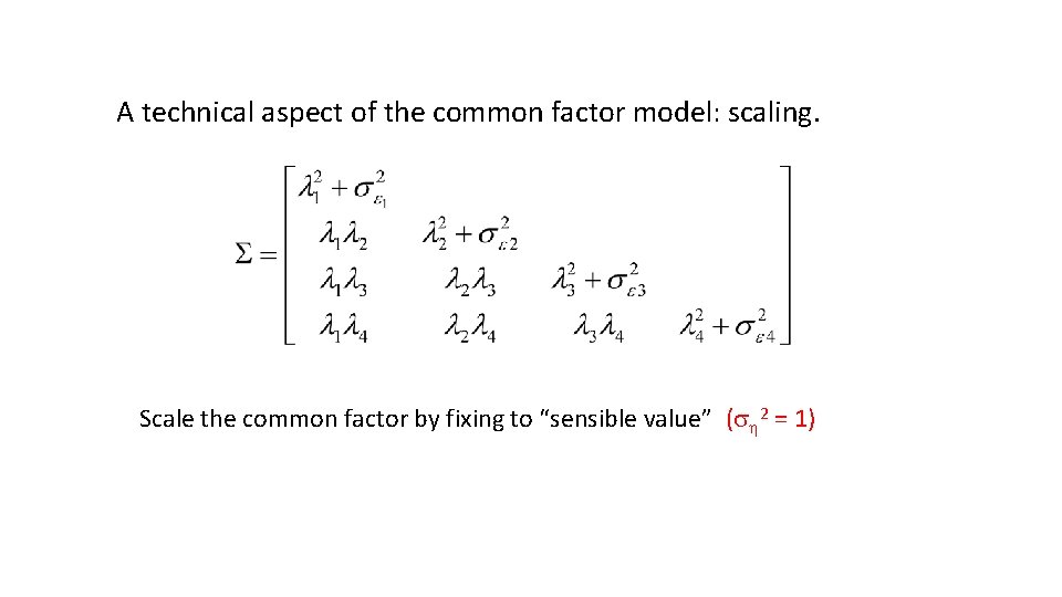
# datf=read. table('rdataf') colnames(datf)=c('sex', 'n 1', 'n 2', 'n 3', 'n 4', 'n 5', 'n 6', 'e 1', 'e 2', 'e 3', 'e 4', 'e 5', 'e 6', 'o 1', 'o 2', 'o 3', 'o 4', 'o 5', 'o 6', 'a 1', 'a 2', 'a 3', 'a 4', 'a 5', 'a 6', 'c 1', 'c 2', 'c 3', 'c 4', 'c 5', 'c 6') datf_n 4=datf[, 4: 7] Sn 4=cov(datf_n 4) round(Sn 4, 3) fa 1=factanal(covmat=Sn 4, n. obs=361, factors=1) # library(Open. Mx) datf_n 4=as. data. frame(datf_n 4) ny=4 selvars=colnames(datf_n 4) # Rn 4=mx. Matrix(type='Stand', nrow=ny, ncol=ny, free=TRUE, value=. 5, lbound=-. 9, ubound=. 9, name='corn 4') Sdsn 4=mx. Matrix(type='Diag', nrow=ny, ncol=ny, free=TRUE, value=5, name='sdsn 4') Meann 4=mx. Matrix(type='Full', nrow=1, ncol=ny, free=TRUE, value=20, name='men 4') Mk. S=mx. Algebra(expression=sdsn 4%*%corn 4%*%sdsn 4, name='Ssatn 4') modelp 1=mx. Model('part 1', Rn 4, Sdsn 4, Meann 4, Mk. S) # N 4 model 0=mx. Model("N 4 sat", mx. Data( observed=datf, type="raw"), # the data mx. FIMLObjective( covariance="part 1. Ssatn 4", means="part 1. men 4", dimnames=selvars) # the fit function ) Model 1 <- mx. Model("model 1", modelp 1, N 4 model 0, mx. Algebra(N 4 sat. objective, name="minus 2 loglikelihood"), mx. Algebra. Objective("minus 2 loglikelihood")) # fit the model Model 1_o <- mx. Run(Model 1) # Ly=mx. Matrix(type='Full', nrow=ny, ncol=1, free=TRUE, value=1, name='Ly') Te=mx. Matrix(type='Diag', nrow=ny, ncol=ny, free=TRUE, value=5, name='Te') Ps=mx. Matrix(type='Symm', nrow=1, ncol=1, free=FALSE, value=1, name='Ps') Meann 4=mx. Matrix(type='Full', nrow=1, ncol=ny, free=TRUE, value=20, name='men 4') Mk. S=mx. Algebra(expression=Ly%*%Ps%*%t(Ly)+Te, name='S 1 fn 4') # modelp 1=mx. Model('part 1', Ly, Te, Ps, Meann 4, Mk. S) # N 4 model 2=mx. Model("N 4 f 1", mx. Data( observed=datf, type="raw"), # the data mx. FIMLObjective( covariance="part 1. S 1 fn 4", means="part 1. men 4", dimnames=selvars) # the fit function # ) Model 2 <- mx. Model("model 1", modelp 1, N 4 model 2, mx. Algebra(N 4 f 1. objective, name="minus 2 loglikelihood"), mx. Algebra. Objective("minus 2 loglikelihood")) # fit the model Model 2_o <- mx. Run(Model 2) Mx. Compare(Model 1_o, Model 2_o) The chi 2 goodness of fit test (c 2=1. 36, df=2) suggest that the model fits well. The observed covariance structure is consistent with my theory. Does this prove the presence of the latent variable? necessary but not sufficient…. Why df=2? Count the observed statistics (S), and the estimated parameters (P): df = S-P.

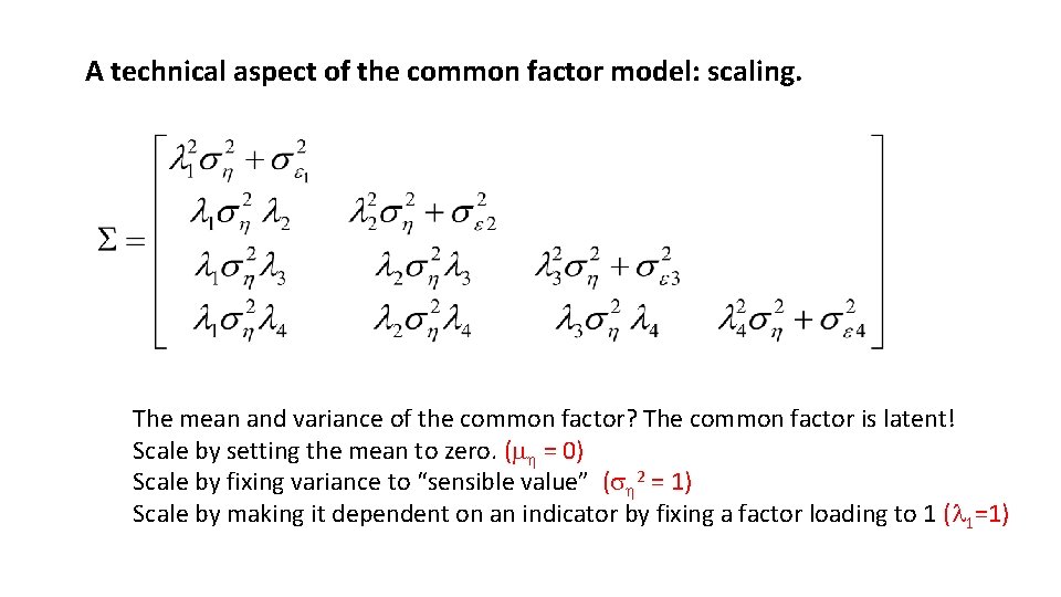
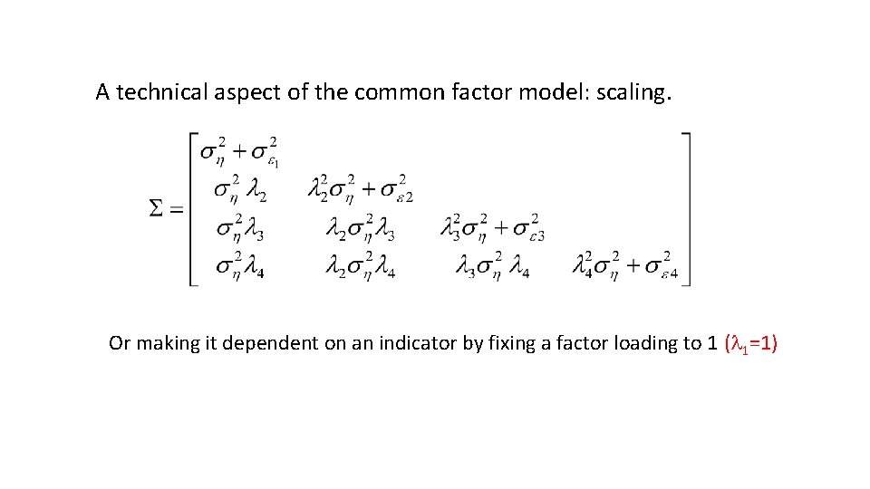
A technical aspect of the common factor model: scaling. The mean and variance of the common factor? The common factor is latent! Scale by setting the mean to zero. (m = 0) Scale by fixing variance to “sensible value” (s 2 = 1) Scale by making it dependent on an indicator by fixing a factor loading to 1 (l 1=1)

But we know about scaling, because this model uses the same scaling (var(E)=var(C)=var(A) = 1; mean(A)=mean(C)=mean(E)=0) MZ=DZ=1 1 E A C e c a T 1 1 MZ=1 / DZ=. 5 1 1 A E C a c e T 2

A technical aspect of the common factor model: scaling. Scale the common factor by fixing to “sensible value” (s 2 = 1)

A technical aspect of the common factor model: scaling. Or making it dependent on an indicator by fixing a factor loading to 1 (l 1=1)

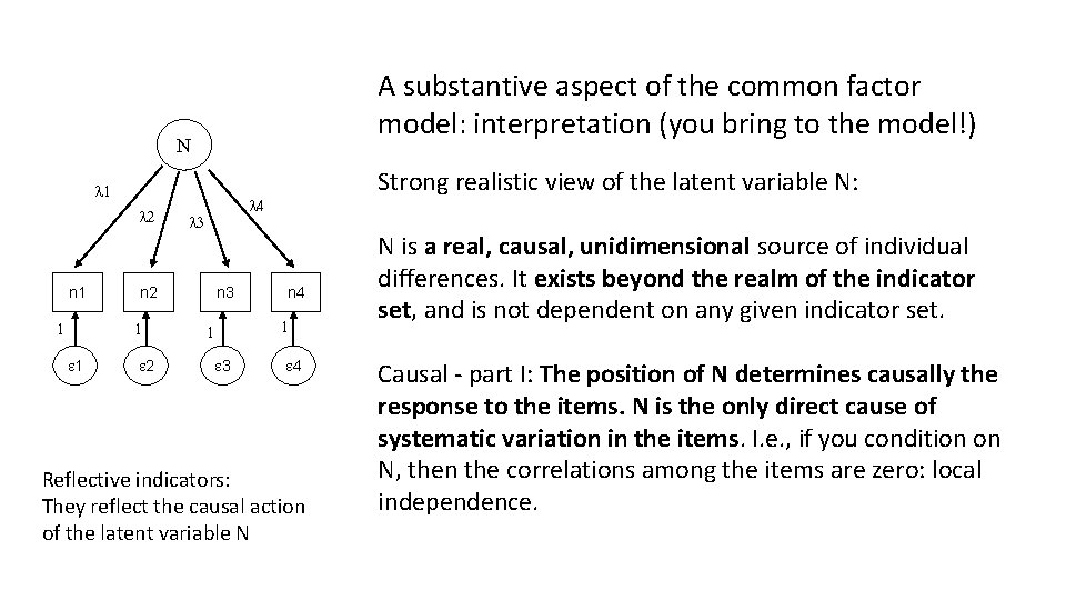
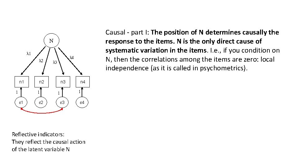
A substantive aspect of the common factor model: interpretation (you bring to the model!) N l 1 l 2 n 1 1 l 4 l 3 n 2 1 1 2 Strong realistic view of the latent variable N: n 3 n 4 1 1 3 4 Reflective indicators: They reflect the causal action of the latent variable N N is a real, causal, unidimensional source of individual differences. It exists beyond the realm of the indicator set, and is not dependent on any given indicator set. Causal - part I: The position of N determines causally the response to the items. N is the only direct cause of systematic variation in the items. I. e. , if you condition on N, then the correlations among the items are zero: local independence.

Causal - part I: The position of N determines causally the response to the items. N is the only direct cause of systematic variation in the items. I. e. , if you condition on N, then the correlations among the items are zero: local independence (as it is called in psychometrics). N l 1 l 2 n 1 1 l 3 n 2 1 1 l 4 2 n 3 n 4 1 1 3 4 Reflective indicators: They reflect the causal action of the latent variable N

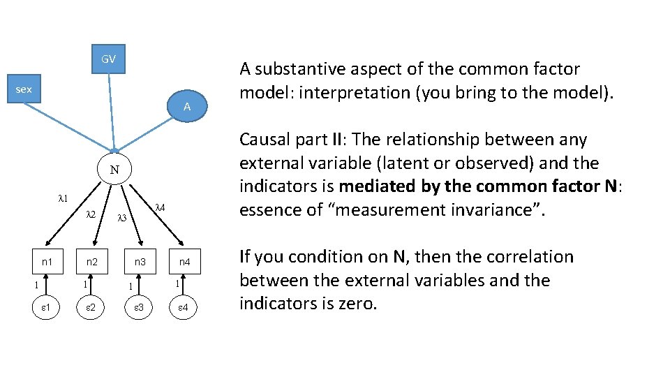
GV sex A Causal part II: The relationship between any external variable (latent or observed) and the indicators is mediated by the common factor N: essence of “measurement invariance”. N l 1 l 2 n 1 n 2 1 1 1 l 4 l 3 2 n 3 n 4 1 1 3 A substantive aspect of the common factor model: interpretation (you bring to the model). 4 If you condition on N, then the correlation between the external variables and the indicators is zero.

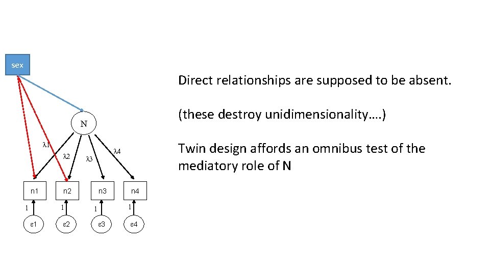
sex Direct relationships are supposed to be absent. (these destroy unidimensionality…. ) N l 1 l 2 n 1 1 l 3 n 2 1 1 2 Twin design affords an omnibus test of the mediatory role of N l 4 n 3 n 4 1 1 3 4

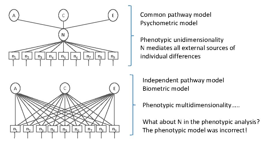
C A E N n 1 n 2 n 3 n 4 n 5 n 6 n 7 n 8 C A n 9 E Common pathway model Psychometric model Phenotypic unidimensionality N mediates all external sources of individual differences Independent pathway model Biometric model Phenotypic multidimensionality…. . n 1 n 2 n 3 n 4 n 5 n 6 n 7 n 8 n 9 What about N in the phenotypic analysis? The phenotypic model was incorrect!

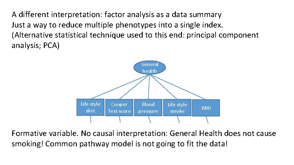
A different interpretation: factor analysis as a data summary Just a way to reduce multiple phenotypes into a single index. (Alternative statistical technique used to this end: principal component analysis; PCA) General health Life style diet Cooper Test score Blood pressure Life style smoke BMI Formative variable. No causal interpretation: General Health does not cause smoking! Common pathway model is not going to fit the data!

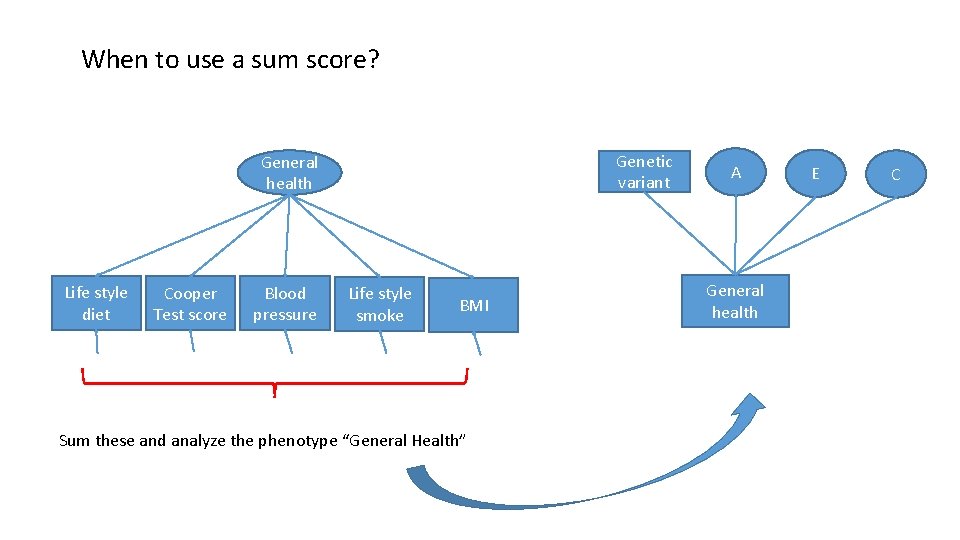
When to use a sum score? Genetic variant General health Life style diet Cooper Test score Blood pressure Life style smoke BMI Sum these and analyze the phenotype “General Health” A General health E C

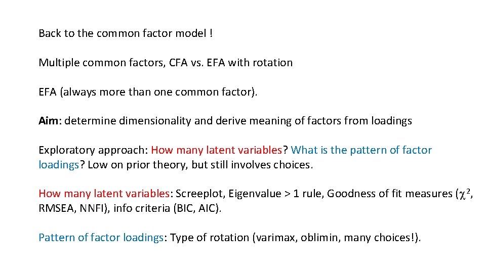
Back to the common factor model ! Multiple common factors, CFA vs. EFA with rotation EFA (always more than one common factor). Aim: determine dimensionality and derive meaning of factors from loadings Exploratory approach: How many latent variables? What is the pattern of factor loadings? Low on prior theory, but still involves choices. How many latent variables: Screeplot, Eigenvalue > 1 rule, Goodness of fit measures (c 2, RMSEA, NNFI), info criteria (BIC, AIC). Pattern of factor loadings: Type of rotation (varimax, oblimin, many choices!).

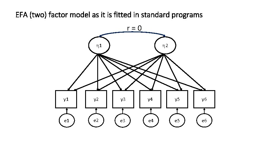
EFA (two) factor model as it is fitted in standard programs r=0 1 2 y 1 y 2 y 3 y 4 y 5 y 6 e 1 e 2 e 3 e 4 e 5 e 6

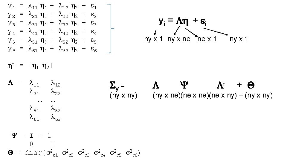
y 1 = l 11 1 + l 12 2 + 1 y 2 = l 21 1 + l 22 2 + 2 y 3 = l 31 1 + l 32 2 + 3 y 4 = l 41 1 + l 42 2 + 4 y 5 = l 51 1 + l 52 2 + 5 y 6 = l 61 1 + l 62 2 + 6 t = [ 1 2] = l 11 l 12 l 21 l 22 … … l 51 l 52 l 61 l 62 yi = i + i ny x 1 ny x ne ne x 1 Sy = (ny x ny) Y = I = 1 0 1 Q = diag(s 2 1 s 2 2 s 2 3 s 2 4 s 2 5 s 2 6) Y t ny x 1 + Q (ny x ne)(ne x ny) + (ny x ny)

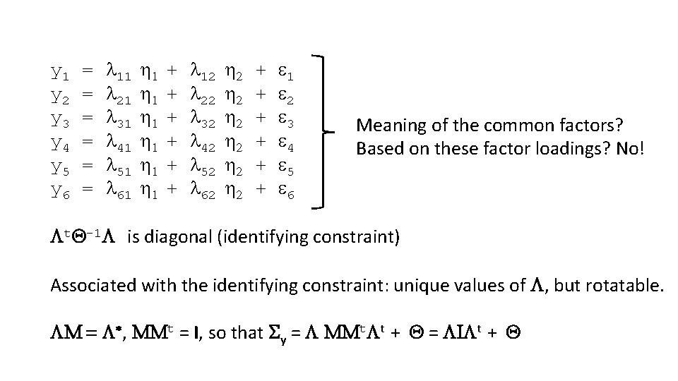
y 1 = l 11 1 + l 12 2 + 1 y 2 = l 21 1 + l 22 2 + 2 y 3 = l 31 1 + l 32 2 + 3 y 4 = l 41 1 + l 42 2 + 4 y 5 = l 51 1 + l 52 2 + 5 y 6 = l 61 1 + l 62 2 + 6 Meaning of the common factors? Based on these factor loadings? No! t. Q-1 is diagonal (identifying constraint) Associated with the identifying constraint: unique values of , but rotatable. M = *, MMt = I, so that Sy = MMt t + Q = I t + Q

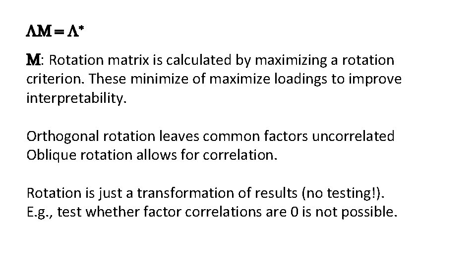
M = * M: Rotation matrix is calculated by maximizing a rotation criterion. These minimize of maximize loadings to improve interpretability. Orthogonal rotation leaves common factors uncorrelated Oblique rotation allows for correlation. Rotation is just a transformation of results (no testing!). E. g. , test whether factor correlations are 0 is not possible.

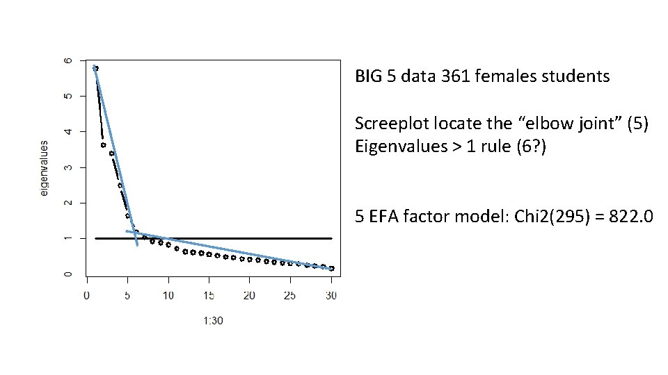
BIG 5 data 361 females students Screeplot locate the “elbow joint” (5) Eigenvalues > 1 rule (6? ) 5 EFA factor model: Chi 2(295) = 822. 0

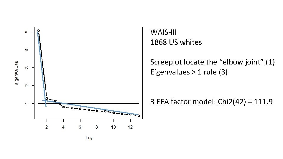
WAIS-III 1868 US whites Screeplot locate the “elbow joint” (1) Eigenvalues > 1 rule (3) 3 EFA factor model: Chi 2(42) = 111. 9

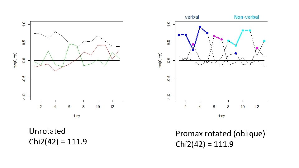
verbal Unrotated Chi 2(42) = 111. 9 Non-verbal Promax rotated (oblique) Chi 2(42) = 111. 9

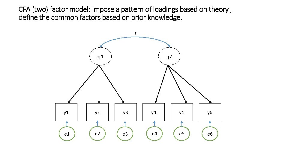
CFA (two) factor model: impose a pattern of loadings based on theory , define the common factors based on prior knowledge. r 1 2 y 1 y 2 y 3 y 4 y 5 y 6 e 1 e 2 e 3 e 4 e 5 e 6

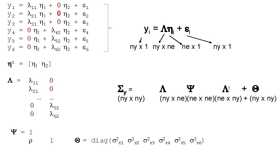
y 1 = l 11 1 + 0 2 + 1 y 2 = l 21 1 + 0 2 + 2 y 3 = l 31 1 + 0 2 + 3 y 4 = 0 1 + l 42 2 + 4 y 5 = 0 1 + l 52 2 + 5 y 6 = 0 1 + l 62 2 + 6 t = [ 1 2] = l 11 0 l 21 0 … … 0 l 52 0 l 62 yi = i + i ny x 1 ny x ne ne x 1 Sy = (ny x ny) Y 1 t + Q (ny x ne)(ne x ny) + (ny x ny) Y = 1 r ny x 1 Q = diag(s 2 1 s 2 2 s 2 3 s 2 4 s 2 5 s 2 6)

Sy = (ny x ny) Y t + Q (ny x ne)(ne x ny) + (ny x ny) In CFA, in contrast to EFA, you can impose all kinds of constraints on the parameters In CFA, in constrast to EFA, you can estimate off-diagonal elements in the cov matrix of the residuals Q

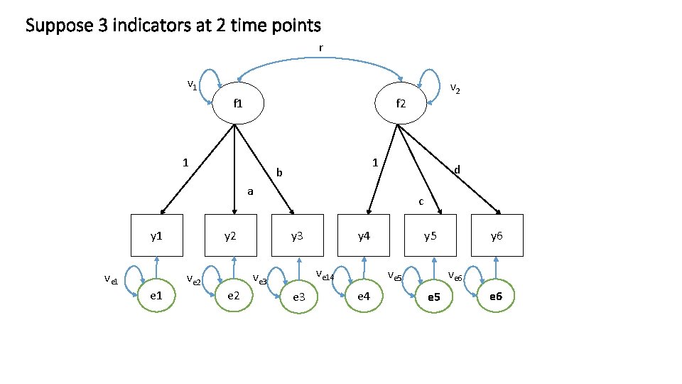
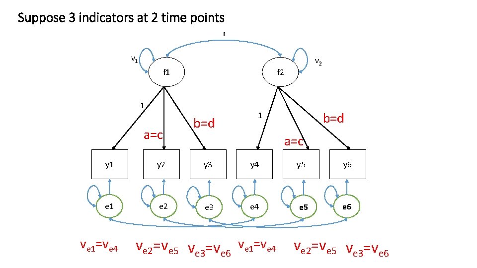
Suppose 3 indicators at 2 time points r v 1 f 2 1 1 b d a y 1 ve 1 y 2 e 1 c y 3 e 2 y 4 ve 14 ve 3 ve 2 v 2 e 3 y 5 ve 6 ve 5 e 4 y 6 e 5 e 6

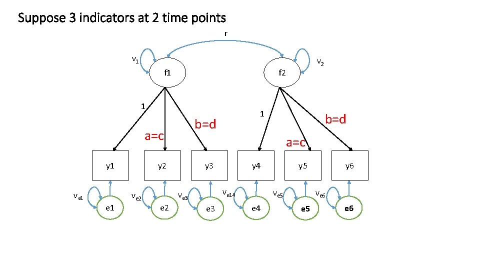
Suppose 3 indicators at 2 time points r v 1 f 2 1 ve 1 y 3 y 4 ve 14 ve 3 e 2 b=d a=c y 2 ve 2 1 b=d a=c y 1 v 2 e 3 y 5 ve 6 ve 5 e 4 y 6 e 5 e 6

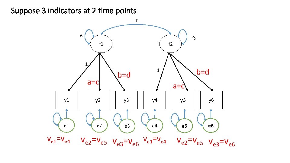
Suppose 3 indicators at 2 time points r v 1 f 2 1 a=c v 2 b=d 1 a=c y 1 y 2 y 3 y 4 y 5 y 6 e 1 e 2 e 3 e 4 e 5 e 6 ve 1=ve 4 ve 2=ve 5 ve 3=ve 6

Suppose 3 indicators at 2 time points r v 1 f 2 1 a=c v 2 b=d 1 a=c y 1 y 2 y 3 y 4 y 5 y 6 e 1 e 2 e 3 e 4 e 5 e 6 ve 1=ve 4 ve 2=ve 5 ve 3=ve 6

MZ=DZ=1 1 E A C e c a 1 MZ=1 / DZ=. 5 1 1 A E C a T 1 c e T 2 Equality constraints are nothing new!

The linear common factor model: “continuous” indicators (7 point Likert scale is “continuous”) What about ordinal or binary indicators? Linear regression model is key ingredient in the linear factor model Logistic or probit regression is a key ingredient in ordinal or discrete factor analysis.

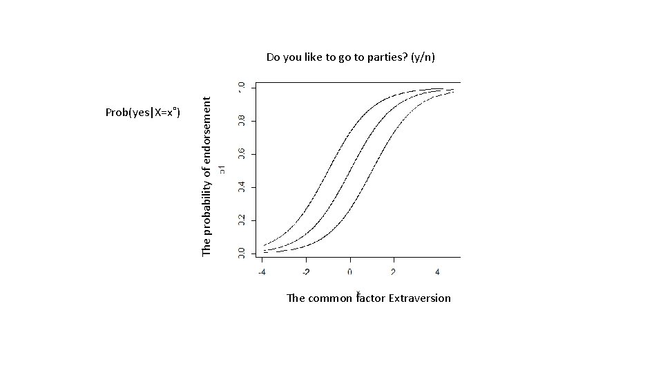
The model for the Yi = b 0 + b 1*Xi + ei E[Y|X=x˚] = b 0 + b 1*x˚ Logit: E[Z|X=x˚] = Prob(Z=0|X=x˚) = exp(b 0 + b 1*x˚) / {1 + exp(b 0 + b 1*x˚)} Probit: E[Z|X=x˚] = Prob(Z=0|X=x˚) = F(b 0 + b 1*x˚), F(. ) cumulative st. normal distribution Replace X, observed predictor, but , the common factor.

Prob(yes|X=x˚) The probability of endorsement Do you like to go to parties? (y/n) The common factor Extraversion