Factor Analysis Structural Equations Model 16 Factor Analysis


 • Generate two variables correlating each other. – 2変数(相互に相関を持つ)の発生 rho <-")
 • More than 3 variables with given correlation coef.")
 Generation for example data # p 308 generation of data for factor")
 eval <- data. frame(subjects) plot(eval)")
 corrcoef jap soc math sci eng jap")
![因子数の決定(相関係数の固有値) Eigen Value of Correlation Coef. Matrix eigen(corrcoef) $values [1] 2. 5577515 1. 0654064](https://slidetodoc.com/presentation_image_h/147a87b70a7a3e4b7b55990e21e217ff/image-9.jpg "因子数の決定(相関係数の固有値) Eigen Value of Correlation Coef. Matrix eigen(corrcoef) $values [1] 2. 5577515 1. 0654064")
 fvarimax <- factanal(subjects, factors=2, scores=\"regression\") print(fvarimax, cutoff=0) Uniquenesses: 国語 社会 数学 理科 英語")
![plot(fvarimax$loadings[, 1], fvarimax$loadings[, 2], asp=1) abline(h=0, v=0) text(fvarimax$loadings[, 1], fvarimax$loadings[, 2], labels=c("jap", "soc", "math",](https://slidetodoc.com/presentation_image_h/147a87b70a7a3e4b7b55990e21e217ff/image-11.jpg "plot(fvarimax$loadings[, 1], fvarimax$loadings[, 2], asp=1) abline(h=0, v=0) text(fvarimax$loadings[, 1], fvarimax$loadings[, 2], labels=c(\"jap\", \"soc\", \"math\",")
![# fvarimax <- factanal(subjects, factors=2, scores="regression") plot(fvarimax$score[, 1], fvarimax$score[, 2], asp=1) abline(h=0, v=0)](https://slidetodoc.com/presentation_image_h/147a87b70a7a3e4b7b55990e21e217ff/image-12.jpg "# fvarimax <- factanal(subjects, factors=2, scores=\"regression\") plot(fvarimax$score[, 1], fvarimax$score[, 2], asp=1) abline(h=0, v=0)")
 fpromax <- factanal(subjects, factors=2, rotation=\"promax\", scores=\"regression\") print(fpromax, cutoff=0, sort=TRUE) 科目 第 1因 第")
![plot(fpromax$loadings[, 1], fpromax$loadings[, 2], asp=1) abline(h=0, v=0) text(fpromax$loadings[, 1], fpromax$loadings[, 2], labels=c("jap", "soc", "math",](https://slidetodoc.com/presentation_image_h/147a87b70a7a3e4b7b55990e21e217ff/image-14.jpg "plot(fpromax$loadings[, 1], fpromax$loadings[, 2], asp=1) abline(h=0, v=0) text(fpromax$loadings[, 1], fpromax$loadings[, 2], labels=c(\"jap\", \"soc\", \"math\",")
 factnorot <- factanal(subjects, factors=2, rotation=\"none\", scores=\"regression\") print(factnorot, cutoff=0) Uniquenesses: jap soc math sci")
![plot(factnorot$loadings[, 1], factnorot$loadings[, 2], asp=1) abline(h=0, v=0) text(factnorot$loadings[, 1], factnorot$loadings[, 2], labels=c("jap", "soc", "math",](https://slidetodoc.com/presentation_image_h/147a87b70a7a3e4b7b55990e21e217ff/image-16.jpg "plot(factnorot$loadings[, 1], factnorot$loadings[, 2], asp=1) abline(h=0, v=0) text(factnorot$loadings[, 1], factnorot$loadings[, 2], labels=c(\"jap\", \"soc\", \"math\",")


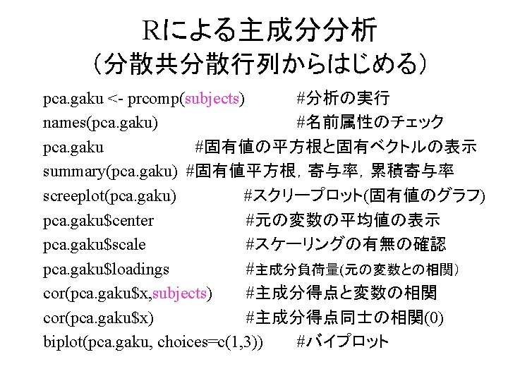
![Rによる主成分分析 (分散共分散行列からはじめる) pca. gaku #固有値の平方根と固有ベクトルの表示 Standard deviations: [1] 13. 971074 9. 674429 6.](https://slidetodoc.com/presentation_image_h/147a87b70a7a3e4b7b55990e21e217ff/image-23.jpg "Rによる主成分分析 (分散共分散行列からはじめる) pca. gaku #固有値の平方根と固有ベクトルの表示 Standard deviations: [1] 13. 971074 9. 674429 6.")
 summary(pca. gaku) #固有値平方根,寄与率,累積寄与率 Importance of components: PC 1 Standard deviation 13.")
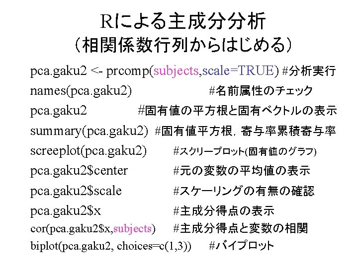
![Rによる主成分分析 (相関係数行列からはじめる) pca. gaku 2 #固有値の平方根と固有ベクトルの表示 Standard deviations: [1] 1. 5992972 1. 0321853](https://slidetodoc.com/presentation_image_h/147a87b70a7a3e4b7b55990e21e217ff/image-27.jpg "Rによる主成分分析 (相関係数行列からはじめる) pca. gaku 2 #固有値の平方根と固有ベクトルの表示 Standard deviations: [1] 1. 5992972 1. 0321853")
 summary(pca. gaku 2) #固有値平方根,寄与率,累積寄与率 Importance of components: PC 1 Standard deviation")
 Linear Structure 観測変数 Observed V. 潜在変数 Latent V. 一般線形構造 General Structure e")
 Linear Structure 観測変数 Observed V. 潜在変数 Latent V. 一般線形構造 δ 2 e 1")
 SEM (Structual Equations Model) • From Package Menu メニューから")
 Specify The Correlation Coefficient Matrix # p 312 specify the correlation coefficient")
 Specify The Correlation Coefficient Matrix (Alt) # p 312 specify the correlation")
 model. coop <- specify. Model() mother -> y 1, b")
 変数 -> 影響先, 推定母数,固定母数 variable -> variable , estimated, fixed model. coop <-")
 内生変数の分散(変数<->変数), 推定母数, 固定母数 Variance of Endogenous Variables variable <-> variable, estimated")
 sem. coop <- sem(model. coop, coopd, N=50) 推定結果の表示 Show")
 Std. Estimate 1 b 11 0. 42983883")
 Model Chisquare = 74. 298 Df = 52 Pr(>Chisq) = 0.")

 Lavaan (latent variable analysis) # From Package Menu メニューから")
 structural")
 summary(result 2,")
 lavaan (0. 5 -11) converged normally after 45")


 data(study) R. study <- cor(study) model. study <- specify. Model() time -> x")

 関数は,変数 がカテゴリー変数であれば,自動的に順位関 係を意味するポリコリック相関係数を算出する –")
 library(sem) data(study) library(polycor) print(R. study <- hetcor(study, std. err=FALSE)$correlations) model. CNES <-")
 = 6. 140618 e-08 Goodness-of-fit")
 sem. Paths(sem. CNES, what=\"stand\", pos. Col=\"black\", fade=FALSE)")

- Slides: 57
因子分析,共分散構造分析 Factor Analysis Structural Equations Model 第 16章 因子分析 Factor Analysis 主成分分析 Principal Components 第 17章 共分散構造分析 Structural Equations Model (SEM)
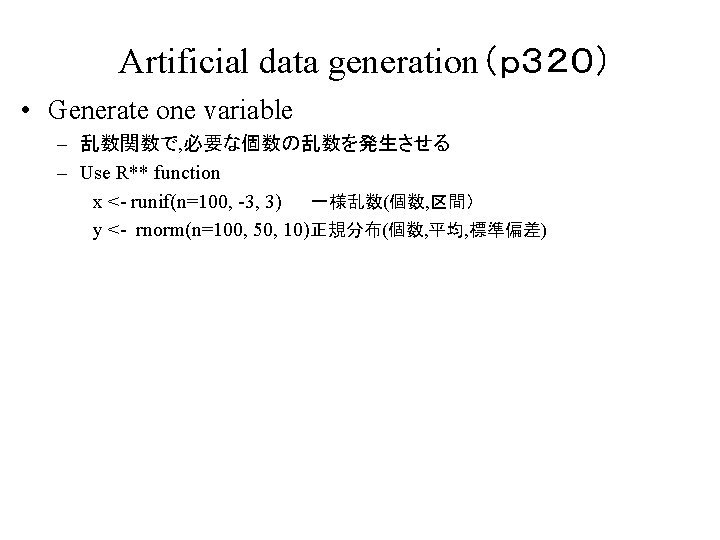
Artificial data generation(p320) • Generate two variables correlating each other. – 2変数(相互に相関を持つ)の発生 rho <- 0. 6 x <-rnorm(100, 50, 10) e <-rnorm(100, 0, 5) y <- rho * x + sqrt(1 -rho^2)*e a 1 <- sqrt(0. 6) a 2 <- sqrt(0. 6) x <- rnorm(100,50,10) e 1 <-rnorm(100, 0, 5) e 2 <-rnorm(100, 0, 5) y 1 <- a 1 *x +sqrt(1 -a 1^2)*e 1 y 2 <- a 2 *x +sqrt(1 -a 2^2)*e 2
Artificial data generation (p 328) • More than 3 variables with given correlation coef. matrix 3変数以 上の発生(任意の相関行列) – 独立乱数からなる行列をZとする. – 母相関行列をRとする. – R=U'U (コレスキー分解) ただしU:上三角行列 – Cholesky decomposition – X =ZU+μ により,目的の人 データができる. ssize <- 10000 vnum <- 4 zz <- matrix(rnorm(n=ssize*vnum), nrow=ssize) meanmat <- matrix(rep(c(1, 2, 3, 4), ssize), nrow=ssize, byrow=TRUE) covar <- matrix(c(1. 0, 0. 5, 0. 4, 0. 3, 0. 5, 1. 0, 0. 5, 0. 4, 0. 5, 1. 0, 0. 5, 0. 3, 0. 4, 0. 5, 1. 0), nrow=vnum) utrngl <- chol(covar) X <- zz %*% utrngl + meanmat mean(X[, 1]) cov(X)
因子分析用データの発生(p 308) Generation for example data # p 308 generation of data for factor analysis set. seed(9999) n <- 200 relation <- matrix(c(0. 09884, 0. 17545, 0. 52720, 0. 73462, 0. 45620, 0. 72141, 0. 47258, 0. 17901, 0. 07984, 0. 37204), nrow=5) indiv <- diag(sqrt(c(0. 53201, 0. 254119, 0. 309986, 0. 546036, 0. 346539))) factpoint <- matrix(rnorm(2*n), nrow=2) indivpt <- matrix(rnorm(5*n), nrow=5) subjects <- round(t(relation%*%factpoint + indiv%*% indivpt)*10+50) colnames(subjects) <- c("jap", "soc", "math", "sci", "eng")
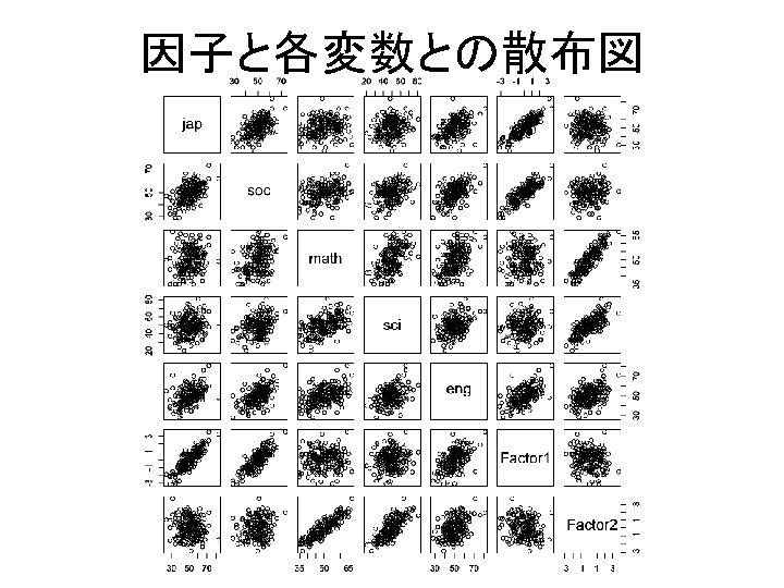
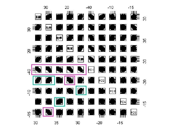
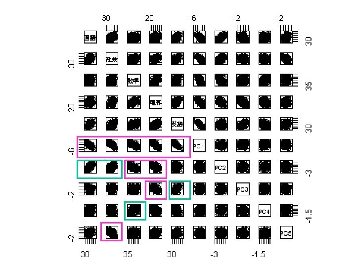
散布図行列 plot(dataframe) eval <- data. frame(subjects) plot(eval)
相関行列 Correlation Coefficients Matrix corrcoef <- cor(subjects) corrcoef jap soc math sci eng jap 1. 000000 0. 550266 0. 195810 0. 163143 0. 4277273 soc 0. 550266 1. 000000 0. 331753 0. 294493 0. 5178159 math 0. 195810 0. 331753 1. 000000 0. 530113 0. 4575891 sci 0. 163143 0. 294493 0. 530113 1. 000000 0. 3876493 eng 0. 427727 0. 517815 0. 457589 0. 387649 1. 0000000
因子数の決定(相関係数の固有値) Eigen Value of Correlation Coef. Matrix eigen(corrcoef) $values [1] 2. 5577515 1. 0654064 0. 5057871 0. 4462341 0. 4248208 Number of eigen values larger than 1. → 2 factors $vectors [, 1] [, 2] [, 3] [, 4] [, 5] [1, ] -0. 4041725 0. 57887716 -0. 3519510 -0. 3105217 0. 53033259 [2, ] -0. 4791143 0. 36327064 -0. 1060289 0. 0743595 -0. 78848747 [3, ] -0. 4380351 -0. 48389701 0. 2494864 -0. 7130299 -0. 05756589 [4, ] -0. 4064104 -0. 54428764 -0. 6058969 0. 3977507 0. 11517295 [5, ] -0. 5000499 0. 05030239 0. 6599499 0. 4810715 0. 28364804
因子分析の実行(直交回転) fvarimax <- factanal(subjects, factors=2, scores="regression") print(fvarimax, cutoff=0) Uniquenesses: 国語 社会 数学 理科 英語 0. 471 0. 395 0. 379 0. 547 0. 491 Loadings: Factor 1 Factor 2 国語 0. 722 0. 085 社会 0. 730 0. 268 数学 0. 177 0. 768 理科 0. 156 0. 655 英語 0. 537 0. 469 Factor 1 Factor 2 SS loadings 1. 399 1. 317 Proportion Var 0. 280 0. 263 Cumulative Var 0. 280 0. 543 jap 第 1因 第 2因 独自 性 子 子 0. 722 0. 085 0. 471 soc 0. 730 0. 268 0. 395 eng 0. 537 0. 469 0. 491 math 0. 177 0. 768 0. 379 Sci 0. 156 0. 469 0. 547 loadings 1. 399 1. 317 科目 Test of the hypothesis that 2 factors are sufficient. The chi square statistic is 0. 08 on 1 degree of freedom. The p-value is 0. 779
plot(fvarimax$loadings[, 1], fvarimax$loadings[, 2], asp=1) abline(h=0, v=0) text(fvarimax$loadings[, 1], fvarimax$loadings[, 2], labels=c("jap", "soc", "math", "sci", "eng"), pos=3)
# fvarimax <- factanal(subjects, factors=2, scores="regression") plot(fvarimax$score[, 1], fvarimax$score[, 2], asp=1) abline(h=0, v=0)
因子分析の実行(斜交回転) fpromax <- factanal(subjects, factors=2, rotation="promax", scores="regression") print(fpromax, cutoff=0, sort=TRUE) 科目 第 1因 第 2因 独自 性 子 子 0. 801 -0. 156 0. 471 Uniquenesses: jap soc math sci eng jap 0. 471 0. 395 0. 379 0. 547 0. 491 Loadings: soc 0. 749 Factor 1 Factor 2 jap 0. 801 -0. 156 eng 0. 461 soc 0. 749 0. 050 math -0. 050 0. 814 math -0. 050 sci -0. 038 0. 693 -0. 038 sci eng 0. 461 0. 348 Factor 1 Factor 2 loadings 1. 419 SS loadings 1. 419 1. 291 Proportion Var 0. 284 0. 258 Cumulative Var 0. 284 0. 542 Test of the hypothesis that 2 factors are sufficient. The chi square statistic is 0. 08 on 1 degree of freedom. The p-value is 0. 779 0. 050 0. 395 0. 348 0. 491 0. 814 0. 379 0. 693 0. 547 1. 291
plot(fpromax$loadings[, 1], fpromax$loadings[, 2], asp=1) abline(h=0, v=0) text(fpromax$loadings[, 1], fpromax$loadings[, 2], labels=c("jap", "soc", "math", "sci", "eng"), pos=3) plot(fpromax$score[, 1], fpromax$score[, 2], asp=1) abline(h=0, v=0)
因子分析の実行(無回転) factnorot <- factanal(subjects, factors=2, rotation="none", scores="regression") print(factnorot, cutoff=0) Uniquenesses: jap soc math sci eng 0. 471 0. 395 0. 379 0. 547 0. 491 Loadings: Factor 1 Factor 2 jap 0. 583 -0. 435 soc 0. 715 -0. 307 math 0. 656 0. 436 sci 0. 563 0. 369 eng 0. 713 -0. 028 Factor 1 Factor 2 SS loadings 2. 106 0. 610 Proportion Var 0. 421 0. 122 Cumulative Var 0. 421 0. 543 科目 第 1 因子 第 2 独自 因子 性 jap 0. 583 -0. 435 0. 471 soc 0. 715 -0. 307 0. 395 eng 0. 656 0. 436 0. 379 math 0. 563 0. 369 0. 547 Sci 0. 713 -0. 028 0. 491 loadings 2. 106 0. 610 Test of the hypothesis that 2 factors are sufficient. The chi square statistic is 0. 08 on 1 degree of freedom. The p-value is 0. 779
plot(factnorot$loadings[, 1], factnorot$loadings[, 2], asp=1) abline(h=0, v=0) text(factnorot$loadings[, 1], factnorot$loadings[, 2], labels=c("jap", "soc", "math", "sci", "eng"), pos=3) plot(factnorot$score[, 1], factnorot$score[, 2], asp=1) abline(h=0, v=0)
因子得点の算出 Factor Score for each sample • 因子負荷量と各個体のデータから算出 – 不確定性があり,複数の方法がある • バートレットの重み付き最小二乗法 • トムソンの回帰推定法 – factoanal(df, factors=n, scores="Bartlett", "regression", "none") ffive <- factanal(subjects, factors=2, scores="Bartlett") score <- data. frame(cbind(subjects, ffive$scores)) plot(score)
Rによる主成分分析 (分散共分散行列からはじめる) pca. gaku #固有値の平方根と固有ベクトルの表示 Standard deviations: [1] 13. 971074 9. 674429 6. 556847 5. 395683 5. 088521 Rotation: PC 1 PC 2 PC 3 PC 4 PC 5 国語 -0. 4545261 0. 6634739 -0. 47289752 0. 14516839 0. 32939713 社会 -0. 3667710 0. 2531514 0. 07138947 -0. 05134978 -0. 89087609 数学 -0. 3561308 -0. 2524045 0. 28362861 0. 85244739 0. 04848823 理科 -0. 5479742 -0. 6486996 -0. 45243098 -0. 27164715 0. 02066735 英語 -0. 4814356 0. 1058187 0. 69723203 -0. 41932160 0. 30831653
Rによる主成分分析 (分散共分散行列からはじめる) summary(pca. gaku) #固有値平方根,寄与率,累積寄与率 Importance of components: PC 1 Standard deviation 13. 971 Proportion of Variance 0. 505 Cumulative Proportion 0. 505 PC 2 9. 674 0. 242 0. 747 PC 3 6. 557 0. 111 0. 858 PC 4 5. 3957 0. 0753 0. 9331 PC 5 5. 089 0. 067 1. 000 cor(pca. gaku$x, subjects) #主成分負荷量:得点と原変数の相関 国語 社会 数学 理科 英語 PC 1 -0. 65302293 -0. 70318791 -0. 66851161 -0. 73343826 -0. 7778664 PC 2 0. 66006849 0. 33608746 -0. 32808926 -0. 60123277 0. 1183926 PC 3 -0. 31886138 0. 06423561 0. 24987036 -0. 28419803 0. 5287002 PC 4 0. 08054865 -0. 03802171 0. 61799311 -0. 14041879 -0. 2616560 PC 5 0. 17236584 -0. 62209333 0. 03315107 0. 01007511 0. 1814368
Rによる主成分分析 (相関係数行列からはじめる) pca. gaku 2 #固有値の平方根と固有ベクトルの表示 Standard deviations: [1] 1. 5992972 1. 0321853 0. 7111871 0. 6680076 0. 6517828 Rotation: PC 1 PC 2 PC 3 PC 4 PC 5 国語 -0. 4041725 0. 57887716 -0. 3519510 0. 3105217 0. 53033259 社会 -0. 4791143 0. 36327064 -0. 1060289 -0. 0743595 -0. 78848747 数学 -0. 4380351 -0. 48389701 0. 2494864 0. 7130299 -0. 05756589 理科 -0. 4064104 -0. 54428764 -0. 6058969 -0. 3977507 0. 11517295 英語 -0. 5000499 0. 05030239 0. 6599499 -0. 4810715 0. 28364804
Rによる主成分分析 (相関係数行列からはじめる) summary(pca. gaku 2) #固有値平方根,寄与率,累積寄与率 Importance of components: PC 1 Standard deviation 1. 599 Proportion of Variance 0. 512 Cumulative Proportion 0. 512 PC 2 1. 032 0. 213 0. 725 PC 3 0. 711 0. 101 0. 826 PC 4 0. 6680 0. 0892 0. 9150 PC 5 0. 652 0. 085 1. 000 cor(pca. gaku 2$x, subjects) #主成分負荷量:得点と原変数の相関 国語 社会 数学 理科 英語 PC 1 -0. 6463919 -0. 76624613 -0. 70054837 -0. 64997107 -0. 79972835 PC 2 0. 5975085 0. 37496261 -0. 49947137 -0. 56180569 0. 05192139 PC 3 -0. 2503030 -0. 07540635 0. 17743154 -0. 43090611 0. 46934784 PC 4 0. 2074308 -0. 04967271 0. 47630935 -0. 26570047 -0. 32135939 PC 5 0. 3456617 -0. 51392258 -0. 03752046 0. 07506775 0. 18487692
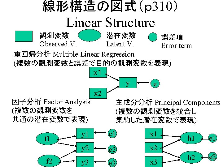
線形構造の図式(p 310) Linear Structure 観測変数 Observed V. 潜在変数 Latent V. 一般線形構造 General Structure e 4 δ 2 f 2 y 4 f 1 e 5 y 5 f 3 誤差項 Error term y 1 e 1 y 2 e 2 y 3 e 3 Structural Equation Model (SEM), δ 3 Linear Structure Regression with Latent variables(LISREL)
線形構造の図式(p 310) Linear Structure 観測変数 Observed V. 潜在変数 Latent V. 一般線形構造 δ 2 e 1 f 2 y 1 e 2 y 2 e 3 y 3 e 4 y 4 f 1 f 3 δ 3 誤差項 Error Term y 5 e 5 y 6 y 7 e 6 e 7 y 8 e 8 y 9 e 9 y 10 y 11 e 10 e 11 y 12 e
パッケージを使う Use Additional Package (1) SEM (Structual Equations Model) • From Package Menu メニューから # Select a Mirror Site CRANミラーサイト指定 # install the package プルダウンから選ぶ – Type from Command Line コマンドラインから install. packages("sem") install. packages("sem. Plot") • Make a Library in the Package Effective パッケージ内のライブラリーを有効にする library(sem) library(sem. Plot)
相関係数行列入力(p 312) Specify The Correlation Coefficient Matrix # p 312 specify the correlation coefficient matrix (as lower triangular matrix) coopd<- read. Moments(names=c( "y 1", "y 2", "y 3", "y 4", "y 5", "y 6", "y 7", "y 8", "y 9", "y 10", "y 11", "y 12")) 1. 0. 160 1. 0. 302 . 341 1. 0. 461 . 400 . 372 1. 0. 299 . 404 . 552. 302 1. 0. 152 . 320 . 476. 225. 708 1. 0. 134 . 403 . 467. 256. 623. 324 1. 0. 182 . 374 . 572. 255. 776. 769. 724 1. 0. 251 . 285 . 316. 164. 361. 295. 260. 284 1. 0. 372 . 100 . 408. 236. 294. 206. 071. 142. 295 1. 0. 157 . 291 . 393. 229. 472. 351. 204. 320. 290. 468 1. 0. 206 -0. 014. 369. 224. 342. 202. 152. 189. 418. 351. 385 1. 0
相関係数行列の入力(p 313) Specify The Correlation Coefficient Matrix (Alt) # p 312 specify the correlation coefficient matrix (without diagonal values) coopd <- read. Moments (diag=FALSE, names=as. character(paste("y", 1: 12, sep=""))). 160 . 302. 341 . 461. 400. 372. 299. 404. 552. 302. 152. 320. 476. 225. 708. 134. 403. 467. 256. 623. 324. 182. 374. 572. 255. 776. 769. 724. 251. 285. 316. 164. 361. 295. 260. 284. 372. 100. 408. 236. 294. 206. 071. 142. 295. 157. 291. 393. 229. 472. 351. 204. 320. 290. 468. 206 -. 014 0. 369. 224. 342. 202. 152. 189. 418. 351. 385
SEMpackege Description of Equations 方程式の記述(全体) model. coop <- specify. Model() mother -> y 1, b 11, NA mother-> y 2, b 21, NA mother-> y 3, b 31, NA mother-> y 4, b 41, NA interaction-> y 5, NA, 1 interaction-> y 6, b 62, NA interaction-> y 7, b 72, NA interaction-> y 8, b 82, NA cooperative -> y 9, NA, 1 cooperative -> y 10, b 103, NA cooperative -> y 11, b 113, NA cooperative -> y 12, b 123, NA mother-> interaction, g 21, NA mother-> cooperative, g 31, NA y 1 <-> y 1, e 1, NA y 2 <-> y 2, e 2, NA
Description of Relations(係数の記述) 変数 -> 影響先, 推定母数,固定母数 variable -> variable , estimated, fixed model. coop <- specify. Model() mother -> y 1, b 11, NA mother-> y 2, b 21, NA mother-> y 3, b 31, NA mother-> y 4, b 41, NA interaction-> y 5, NA, 1 interaction-> y 6, b 62, NA interaction-> y 7, b 72, NA interaction-> y 8, b 82, NA cooperative -> y 9, NA, 1 cooperative -> y 10, b 103, NA cooperative -> y 11, b 113, NA cooperative -> y 12, b 123, NA mother-> interaction, g 21, NA mother-> cooperative, g 31, NA
Descrition of Variances(分散の記述) 内生変数の分散(変数<->変数), 推定母数, 固定母数 Variance of Endogenous Variables variable <-> variable, estimated parameter, fixed param. y 1 <-> y 1, e 1, NA y 2 <-> y 2, e 2, NA y 3 <-> y 3, e 3, NA y 4 <-> y 4, e 4, NA y 5 <-> y 5, e 5, NA y 6 <-> y 6, e 6, NA y 7 <-> y 7, e 7, NA y 8 <-> y 8, e 8, NA y 9 <-> y 9, e 9, NA y 10 <-> y 10, e 10, NA y 11 <-> y 11, e 11, NA y 12 <-> y 12, e 12, NA mother<-> mother, NA, 1 interaction<-> interaction, delta 2, NA cooperative <-> cooperative, delta 3, NA
SEM Package 推定母数の計算 sem(モデル名, 相関係数行列,データ数) sem. coop <- sem(model. coop, coopd, N=50) 推定結果の表示 Show the result std. Coef(sem. coop) summary(sem. coop)
SEM Package 標準化解 std. Coef(sem. coop, digit=4) Std. Estimate 1 b 11 0. 42983883 y 1 <--- mother 2 b 21 0. 48778549 y 2 <--- mother 3 b 31 0. 79918897 y 3 <--- mother 4 b 41 0. 52056885 y 4 <--- mother 5 0. 83781298 y 5 <--- interaction 6 b 62 0. 78544837 y 6 <--- interaction 7 b 72 0. 71857356 y 7 <--- interaction 8 b 82 0. 95364525 y 8 <--- interaction 9 0. 54048885 y 9 <--- cooperative 10 b 103 0. 62410058 y 10 <--- cooperative 11 b 113 0. 66941836 y 11 <--- cooperative 12 b 123 0. 59279790 y 12 <--- cooperative 13 g 21 0. 71286901 interaction <--- mother 14 g 31 0. 72109345 cooperative <--- mother 15 e 1 0. 81523858 y 1 <--> y 1 16 e 2 0. 76206532 y 2 <--> y 2 17 e 3 0. 36129699 y 3 <--> y 3 18 e 4 0. 72900807 y 4 <--> y 4 19 e 5 0. 29806940 y 5 <--> y 5 20 e 6 0. 38307086 y 6 <--> y 6 21 e 7 0. 48365204 y 7 <--> y 7 22 e 8 0. 09056074 y 8 <--> y 8 23 e 9 0. 70787180 y 9 <--> y 9 24 e 10 0. 61049846 y 10 <--> y 10 25 e 11 0. 55187906 y 11 <--> y 11 26 e 12 0. 64859064 y 12 <--> y 12 27 1. 0000 mother <--> mother 28 delta 2 0. 49181777 interaction <--> interaction 29 delta 3 0. 48002423 cooperative <--> cooperative
summary(sem. coop) Model Chisquare = 74. 298 Df = 52 Pr(>Chisq) = 0. 022864 Chisquare (null model) = 291. 59 Df = 66 Goodness-of-fit index = 0. 82725 Adjusted goodness-of-fit index = 0. 74087 RMSEA index = 0. 093548 90% CI: (0. 036288, 0. 13902) Bentler-Bonnett NFI = 0. 74519 Tucker-Lewis NNFI = 0. 87454 Bentler CFI = 0. 90115 SRMR = 0. 082692 AIC = 126. 3 AICc = 135. 34 BIC = 176. 01 CAIC = -181. 13 Normalized Residuals Min. 1 st Qu. Median Mean 3 rd Qu. Max. -1. 52000 -0. 28700 0. 00504 0. 02800 0. 32000 1. 62000 R-square for Endogenous Variables y 1 y 2 y 3 y 4 interaction y 5 0. 1848 0. 2379 0. 6387 0. 2710 0. 5082 0. 7019 y 6 y 7 y 8 cooperative y 9 y 10 0. 6169 0. 5163 0. 9094 0. 5200 0. 2921 0. 3895 y 11 y 12 0. 4481 0. 3514 Parameter Estimates Estimate Std Error z value Pr(>|z|) b 11 0. 429839 0. 151463 2. 8379 4. 5410 e-03 y 1 <--- mother b 21 0. 487785 0. 149279 3. 2676 1. 0846 e-03 y 2 <--- mother b 31 0. 799189 0. 136061 5. 8737 4. 2605 e-09 y 3 <--- mother b 41 0. 520569 0. 147932 3. 5190 4. 3323 e-04 y 4 <--- mother b 62 0. 937499 0. 142621 6. 5734 4. 9196 e-11 y 6 <--- interaction b 72 0. 857678 0. 148517 5. 7749 7. 6981 e-09 y 7 <--- interaction b 82 1. 138256 0. 132401 8. 5970 8. 1816 e-18 y 8 <--- interaction b 103 1. 154696 0. 401369 2. 8769 4. 0161 e-03 y 10 <--- cooperative b 113 1. 238543 0. 416601 2. 9730 2. 9493 e-03 y 11 <--- cooperative b 123 1. 096781 0. 391948 2. 7983 5. 1376 e-03 y 12 <--- cooperative g 21 0. 597251 0. 133801 4. 4637 8. 0544 e-06 interaction <--- mother g 31 0. 389743 0. 133059 2. 9291 3. 3995 e-03 cooperative <--- mother e 1 0. 815239 0. 174334 4. 6763 2. 9210 e-06 y 1 <--> y 1 e 2 0. 762065 0. 166733 4. 5706 4. 8641 e-06 y 2 <--> y 2 e 3 0. 361297 0. 130904 2. 7600 5. 7800 e-03 y 3 <--> y 3 e 4 0. 729008 0. 162139 4. 4962 6. 9182 e-06 y 4 <--> y 4 e 5 0. 298069 0. 074691 3. 9907 6. 5882 e-05 y 5 <--> y 5 e 6 0. 383071 0. 088169 4. 3447 1. 3944 e-05 y 6 <--> y 6 e 7 0. 483652 0. 105790 4. 5718 4. 8350 e-06 y 7 <--> y 7 e 8 0. 090561 0. 055202 1. 6405 1. 0090 e-01 y 8 <--> y 8 e 9 0. 707872 0. 165572 4. 2753 1. 9087 e-05 y 9 <--> y 9 e 10 0. 610498 0. 156681 3. 8965 9. 7612 e-05 y 10 <--> y 10 e 11 0. 551879 0. 153089 3. 6050 3. 1220 e-04 y 11 <--> y 11 e 12 0. 648591 0. 159798 4. 0588 4. 9324 e-05 y 12 <--> y 12 delta 2 0. 345222 0. 120587 2. 8628 4. 1986 e-03 interaction <--> interaction delta 3 0. 140229 0. 092747 1. 5120 1. 3055 e-01 cooperative <--> cooperative Iterations = 48
sem. Paths(sem. coop, what="stand", layout="circle", style="lisrel", shape. Man="rectangle", shape. Lat="ellipse", size. Man=3, resid. Scale=9, pos. Col="black", neg. Col="red", fade=FALSE, edge. label. cex=0. 8) Tree Spring
パッケージを使う Use Additional Package (2) Lavaan (latent variable analysis) # From Package Menu メニューから #Select a Mirror Site CRANミラーサイト指定 #Type from Command Line コマンドラインから install. packages(c("lavaan", "psych", "qgraph")) #Make a Library in the Package Effective library(lavaan) library(psych) library(qgraph) 注意:先にSEMパッケージがインストールされていると同じ 名前のライブラリーは上書きされないため,インストールの 前に,rm(sem) として,sem関数を空にしておくと良い
lavaan packege Description of Equations 方程式の記述 {lavaan}パッケージでは以下のような記号の使い方をしています。 • =~ 測定方程式 measurement • ~ 構造方程式(回帰) structural • ~~ 残差の共分散(相関) covariance model. cooplv <- ' mother =~ y 1+y 2+y 3+y 4 interaction =~ y 5+y 6+y 7+y 8 cooperative =~ y 9+y 10+y 11+y 12 interaction ~ mother cooperative ~ mother '
lavaan Package Estimation result 2 <- sem(model. cooplv, sample. cov=coopd, sample. nobs=50) summary(result 2, fit. measures=TRUE, standardized=TRUE)
Estimated result from Lavaan summary(result 2) lavaan (0. 5 -11) converged normally after 45 iterations Number of observations 50 Estimator ML Minimum Function Test Statistic 75. 367 Degrees of freedom 51 P-value (Chi-square) 0. 015 Parameter estimates: Information Expected Standard Errors Standard Estimate Std. err Z-value P(>|z|) Latent variables: mother =~ y 1 1. 000 y 2 1. 136 0. 504 2. 252 0. 024 y 3 1. 874 0. 688 2. 725 0. 006 y 4 1. 196 0. 517 2. 314 0. 021 interaction =~ y 5 1. 000 y 6 0. 944 0. 144 6. 563 0. 000 y 7 0. 869 0. 149 5. 832 0. 000 y 8 1. 156 0. 134 8. 606 0. 000 cooperative =~ y 9 1. 000 y 10 1. 190 0. 408 2. 919 0. 004 y 11 1. 237 0. 416 2. 971 0. 003 y 12 1. 107 0. 394 2. 810 0. 005 Regressions: interaction ~ mother 1. 428 0. 566 2. 524 0. 012 cooperative ~ mother 0. 949 0. 447 2. 122 0. 034 Covariances: interaction ~~ cooperative -0. 041 0. 060 -0. 675 0. 499
Estimated result from Lavaan Variances: y 1 0. 804 0. 169 y 2 0. 753 0. 162 y 3 0. 362 0. 131 y 4 0. 728 0. 158 y 5 0. 305 0. 074 y 6 0. 378 0. 086 y 7 0. 470 0. 101 y 8 0. 077 0. 053 y 9 0. 699 0. 161 y 10 0. 582 0. 151 y 11 0. 550 0. 149 y 12 0. 636 0. 155 mother 0. 176 0. 124 interaction 0. 316 0. 120 cooperative 0. 122 0. 087 sem. Paths(result 2, what="stand", layout="tree", style="lisrel", shape. Man="rectangle", shape. Lat="ellipse", size. Man=3, resid. Scale=9, pos. Col="black", neg. Col="red", fade=FALSE, edge. label. cex=0. 8)
Example of estimation from original data Study of students Time Confidence Expect
stid, x 1, x 2, x 3, x 4, x 5, x 6 1, 5, 6, 2, 3, 36, 31 2, 4, 4, 5, 6, 51, 45 3, 4, 7, 6, 5, 62, 41 4, 5, 5, 5, 4, 50, 28 5, 4, 5, 60, 38 6, 5, 7, 3, 2, 50, 34 7, 5, 6, 3, 5, 45, 31 8, 6, 7, 5, 5, 62, 56 9, 4, 5, 6, 6, 48, 45 10, 4, 5, 5, 4, 44, 35 11, 3, 3, 5, 4, 59, 42 12, 6, 5, 5, 6, 55, 51 13, 5, 6, 4, 5, 57, 40 14, 8, 8, 6, 5, 58, 54 15, 5, 6, 7, 7, 60 16, 5, 6, 7, 6, 58, 53 17, 6, 5, 6, 6, 48, 45 18, 4, 6, 5, 6, 47, 31 19, 3, 4, 5, 4, 32, 23 20, 4, 3, 4, 4, 25, 24 21, 6, 5, 44, 38 22, 4, 5, 6, 4, 45, 40 23, 3, 3, 5, 4, 28, 33 24, 3, 4, 6, 5, 36, 41 25, 6, 7, 4, 5, 45, 39 26, 3, 4, 3, 2, 35, 36 27, 5, 6, 7, 5, 51, 43 28, 5, 6, 3, 4, 54, 48 29, 3, 4, 6, 7, 38, 26 30, 3, 4, 7, 6, 60, 55 Data <- Copy the data on the left And make a dataframe, using it. # From clipboard store in dataframe #for windows study <- read. delim("clipboard", header=TRUE , sep=", ") #for Mac study <- read. delim(pipe("pbpaste") , header=TRUE , sep=", ")
library(sem) data(study) R. study <- cor(study) model. study <- specify. Model() time -> x 1, NA, 1 time -> x 2, b 12, NA expect -> x 3, NA, 1 expect -> x 4, b 22, NA confid -> x 5, NA, 1 confid -> x 6, b 32, NA time -> expect, g 12, NA time -> confid, g 13, NA expect -> confid, g 23, NA x 1 <-> x 1, e 1, NA x 2 <-> x 2, e 2, NA x 3 <-> x 3, e 3, NA x 4 <-> x 4, e 4, NA x 5 <-> x 5, e 5, NA x 6 <-> x 6, e 6, NA time <-> time, delta 1, NA expect <-> expect, delta 2, NA confid <-> confid, delta 3, NA sem. study <- sem(model. study, R. study, N=30) summary(sem. study, fit. indices=c("GFI", "AGFI", "CFI", "RMSEA")) sem. Paths(sem. study, what="stand", pos. Col="black", fade=FALSE, layout="circle")
観測変数か カテコ リ変数て ある例 Rパッケージの中に初めから含まれているCNES というテ ータ。1997 年の カナタ 国政選挙に関連して「伝統的価値観」への態度を調へ るために行われ た郵送式質問紙調査結果て あり,1529 人分のテ ータか 含まれている。 MBSA 2 an ordered factor with levels ’Strongly. Disagree’, ’Agree’, and ’Strongly. Agree’, in response to the statement, "We should be more tolerant of people who choose to live according to their own standards, even if they are very different from our own. " MBSA 7 an ordered factor in response to the statement, "Newer lifestyles are contributing to the breakdown of our society. " MBSA 8 an ordered factor in response to the statement, "The world is always changing and we should adapt our view of moral behaviour to these changes. " MBSA 9 an ordered factor in response to the statement, "This country would have many fewer problems if there were more emphasis on traditional family values. "
• Polycor パッケージを用いて,カテコ リ変 数間のホ リコリック相関係数を計算させ, それに基づいてSEMを計算する. – Polycorパッケージ内のhetcor() 関数は,変数 がカテゴリー変数であれば,自動的に順位関 係を意味するポリコリック相関係数を算出する – MBSA 2 MBSA 7 MBSA 8 MBSA 9 MBSA 2 1. 0000000 -0. 3017953 0. 2820608 -0. 2230010 MBSA 7 -0. 3017953 1. 0000000 -0. 3422176 0. 5449888 MBSA 8 0. 2820608 -0. 3422176 1. 0000000 -0. 3206524 MBSA 9 -0. 2230010 0. 5449888 -0. 3206524 1. 0000000
install. packages("polycor") library(sem) data(study) library(polycor) print(R. study <- hetcor(study, std. err=FALSE)$correlations) model. CNES <- specify. Model(text=" F -> MBSA 2, lam 1, NA F -> MBSA 7, lam 2, NA F -> MBSA 8, lam 3, NA F -> MBSA 9, lam 4, NA F <-> F, NA, 1 MBSA 2 <-> MBSA 2, the 1, NA MBSA 7 <-> MBSA 7, the 2, NA MBSA 8 <-> MBSA 8, the 3, NA MBSA 9 <-> MBSA 9, the 4, NA ") sem. CNES <- sem(model. CNES, R. CNES, N=1529) summary(sem. CNES, fit. indices=c("GFI", "AGFI", "CFI", "RMSEA")) library(sem. Plot) sem. Paths(sem. CNES, what="stand", pos. Col="black", fade=FALSE)
Model Chisquare = 33. 21151 Df = 2 Pr(>Chisq) = 6. 140618 e-08 Goodness-of-fit index = 0. 9893351 Adjusted goodness-of-fit index = 0. 9466755 RMSEA index = 0. 1010603 90% CI: (0. 07261016, 0. 1326084) Bentler CFI = 0. 9680971 Normalized Residuals Min. 1 st Qu. Median Mean 3 rd Qu. Max. -0. 000003 0. 030014 0. 207794 0. 847925 1. 035458 3. 829661 R-square for Endogenous Variables MBSA 2 MBSA 7 MBSA 8 MBSA 9 0. 1516 0. 6052 0. 2197 0. 4717 Parameter Estimates Estimate Std Error z value Pr(>|z|) lam 1 -0. 3893288 0. 02875484 -13. 53959 9. 129553 e-42 lam 2 0. 7779158 0. 02996521 25. 96063 1. 379186 e-148 lam 3 -0. 4686833 0. 02839946 -16. 50325 3. 476906 e-61 lam 4 0. 6867993 0. 02921502 23. 50843 3. 344412 e-122 the 1 0. 8484230 0. 03281416 25. 85539 2. 116244 e-147 the 2 0. 3948470 0. 03567529 11. 06780 1. 797527 e-28 the 3 0. 7803361 0. 03152466 24. 75320 2. 864101 e-135 the 4 0. 5283068 0. 03212698 16. 44434 9. 208875 e-61 lam 1 MBSA 2 <--- F lam 2 MBSA 7 <--- F lam 3 MBSA 8 <--- F lam 4 MBSA 9 <--- F the 1 MBSA 2 <--> MBSA 2 the 2 MBSA 7 <--> MBSA 7 the 3 MBSA 8 <--> MBSA 8 the 4 MBSA 9 <--> MBSA 9 Iterations = 14
library(sem. Plot) sem. Paths(sem. CNES, what="stand", pos. Col="black", fade=FALSE)
Further Complex Model. . • For non-negative data, count data, ratio data, and so on. – Use "Generalized linear link functions" • Such extensions can be easily done with specialized Statistical Packages than R. – Stata, Sーplus, AMOS, ... https: //pairach. com/2011/08/13/r-packages-for-structuralequation-model/ • Open. Mx (Boker et al, 2011) is claimed to be a “ free and open source software for use with R that allows estimation of a wide variety of advanced multivariate statistical models. ” contributed by experts in R and SEM.