Factor Analysis Structural Equations Model 16 Factor Analysis

 Linear Structure 観測変数 Observed V. 潜在変数 Latent V. 一般線形構造 General Structure e")
 Generation for example data # p 308 generation of data for factor")
 eval <- data. frame(subjects) plot(eval)")
 corrcoef 国語 社会 数学 理科 英語 国語")
![因子数の決定(相関係数の固有値) Eigen Value of Correlation Coef. Matrix eigen(corrcoef) $values [1] 2. 5577515 1. 0654064](https://slidetodoc.com/presentation_image_h2/7d3f6c8e6a16edef360ae05be8ebc25a/image-9.jpg "因子数の決定(相関係数の固有値) Eigen Value of Correlation Coef. Matrix eigen(corrcoef) $values [1] 2. 5577515 1. 0654064")
 fvarimax <- factanal(subjects, factors=2, scores=\"regression\") print(fvarimax, cutoff=0) Uniquenesses: 国語 社会 数学 理科 英語")
![plot(fvarimax$loadings[, 1], fvarimax$loadings[, 2], asp=1) abline(h=0, v=0) text(fvarimax$loadings[, 1], fvarimax$loadings[, 2], labels=c("jap", "soc", "math",](https://slidetodoc.com/presentation_image_h2/7d3f6c8e6a16edef360ae05be8ebc25a/image-11.jpg "plot(fvarimax$loadings[, 1], fvarimax$loadings[, 2], asp=1) abline(h=0, v=0) text(fvarimax$loadings[, 1], fvarimax$loadings[, 2], labels=c(\"jap\", \"soc\", \"math\",")
![#fvarimax <- factanal(subjects, factors=2, scores="regression") plot(fvarimax$score[, 1], fvarimax$score[, 2], asp=1) abline(h=0, v=0)](https://slidetodoc.com/presentation_image_h2/7d3f6c8e6a16edef360ae05be8ebc25a/image-12.jpg "#fvarimax <- factanal(subjects, factors=2, scores=\"regression\") plot(fvarimax$score[, 1], fvarimax$score[, 2], asp=1) abline(h=0, v=0)")
 fpromax <- factanal(subjects, factors=2, rotation=\"promax\", scores=\"regression\") print(fpromax, cutoff=0, sort=TRUE) 科目 Uniquenesses: 国語 社会")
![plot(fpromax$loadings[, 1], fpromax$loadings[, 2], asp=1) abline(h=0, v=0) text(fpromax$loadings[, 1], fpromax$loadings[, 2], labels=c("jap", "soc", "math",](https://slidetodoc.com/presentation_image_h2/7d3f6c8e6a16edef360ae05be8ebc25a/image-14.jpg "plot(fpromax$loadings[, 1], fpromax$loadings[, 2], asp=1) abline(h=0, v=0) text(fpromax$loadings[, 1], fpromax$loadings[, 2], labels=c(\"jap\", \"soc\", \"math\",")
 factnorot <- factanal(subjects, factors=2, rotation=\"none\", scores=\"regression\") print(factnorot, cutoff=0) Uniquenesses: 国語 社会 数学 理科")
![plot(factnorot$loadings[, 1], factnorot$loadings[, 2], asp=1) abline(h=0, v=0) text(factnorot$loadings[, 1], factnorot$loadings[, 2], labels=c("jap", "soc", "math",](https://slidetodoc.com/presentation_image_h2/7d3f6c8e6a16edef360ae05be8ebc25a/image-16.jpg "plot(factnorot$loadings[, 1], factnorot$loadings[, 2], asp=1) abline(h=0, v=0) text(factnorot$loadings[, 1], factnorot$loadings[, 2], labels=c(\"jap\", \"soc\", \"math\",")


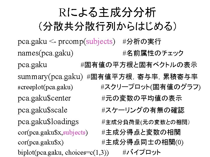
![Rによる主成分分析 (分散共分散行列からはじめる) pca. gaku #固有値の平方根と固有ベクトルの表示 Standard deviations: [1] 13. 971074 9. 674429 6. 556847](https://slidetodoc.com/presentation_image_h2/7d3f6c8e6a16edef360ae05be8ebc25a/image-22.jpg "Rによる主成分分析 (分散共分散行列からはじめる) pca. gaku #固有値の平方根と固有ベクトルの表示 Standard deviations: [1] 13. 971074 9. 674429 6. 556847")
 summary(pca. gaku) #固有値平方根,寄与率,累積寄与率 Importance of components: PC 1 Standard deviation 13. 971")
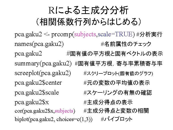
![Rによる主成分分析 (相関係数行列からはじめる) pca. gaku 2 #固有値の平方根と固有ベクトルの表示 Standard deviations: [1] 1. 5992972 1. 0321853 0.](https://slidetodoc.com/presentation_image_h2/7d3f6c8e6a16edef360ae05be8ebc25a/image-26.jpg "Rによる主成分分析 (相関係数行列からはじめる) pca. gaku 2 #固有値の平方根と固有ベクトルの表示 Standard deviations: [1] 1. 5992972 1. 0321853 0.")
 summary(pca. gaku 2) #固有値平方根,寄与率,累積寄与率 Importance of components: PC 1 Standard deviation 1.")
- Slides: 28
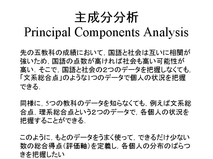
因子分析,共分散構造分析 Factor Analysis Structural Equations Model 第 16章 因子分析 Factor Analysis 主成分分析 Principal Components 第 17章 共分散構造分析 Structural Equations Model (SEM)
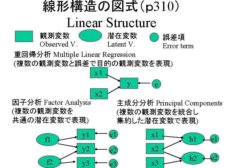
線形構造の図式(p 310) Linear Structure 観測変数 Observed V. 潜在変数 Latent V. 一般線形構造 General Structure e 4 δ 2 f 2 y 4 f 1 e 5 y 5 f 3 誤差項 Error term y 1 e 1 y 2 e 2 y 3 e 3 Structural Equation Model (SEM), δ 3 Linear Structure Regression with Latent variables(LISREL)
因子分析用データの発生(p 308) Generation for example data # p 308 generation of data for factor analysis set. seed(9999) n <- 200 relation <- matrix(c(0. 09884, 0. 17545, 0. 52720, 0. 73462, 0. 45620, 0. 72141, 0. 47258, 0. 17901, 0. 07984, 0. 37204), nrow=5) indiv <- diag(sqrt(c(0. 53201, 0. 254119, 0. 309986, 0. 546036, 0. 346539))) factpoint <- matrix(rnorm(2*n), nrow=2) indivpt <- matrix(rnorm(5*n), nrow=5) subjects <- round(t(relation%*%factpoint + indiv%*% indivpt)*10+50) colnames(subjects) <- c("jap", "soc", "math", "sci", "eng")
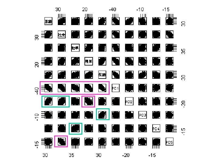
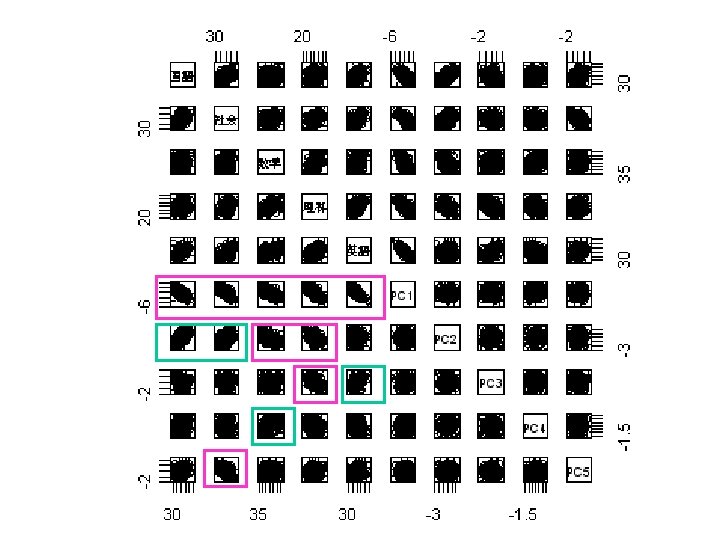
散布図行列 plot(dataframe) eval <- data. frame(subjects) plot(eval)
相関行列 Correlation Coefficients Matrix corrcoef <- cor(subjects) corrcoef 国語 社会 数学 理科 英語 国語 1. 0000000 0. 5502661 0. 1958106 0. 1631430 0. 4277273 社会 0. 5502661 1. 0000000 0. 3317530 0. 2944938 0. 5178159 数学 0. 1958106 0. 3317530 1. 0000000 0. 5301135 0. 4575891 理科 0. 1631430 0. 2944938 0. 5301135 1. 0000000 0. 3876493 英語 0. 4277273 0. 5178159 0. 4575891 0. 3876493 1. 0000000
因子数の決定(相関係数の固有値) Eigen Value of Correlation Coef. Matrix eigen(corrcoef) $values [1] 2. 5577515 1. 0654064 0. 5057871 0. 4462341 0. 4248208 $vectors [, 1] [, 2] [, 3] [, 4] [, 5] [1, ] -0. 4041725 0. 57887716 -0. 3519510 -0. 3105217 0. 53033259 [2, ] -0. 4791143 0. 36327064 -0. 1060289 0. 0743595 -0. 78848747 [3, ] -0. 4380351 -0. 48389701 0. 2494864 -0. 7130299 -0. 05756589 [4, ] -0. 4064104 -0. 54428764 -0. 6058969 0. 3977507 0. 11517295 [5, ] -0. 5000499 0. 05030239 0. 6599499 0. 4810715 0. 28364804
因子分析の実行(直交回転) fvarimax <- factanal(subjects, factors=2, scores="regression") print(fvarimax, cutoff=0) Uniquenesses: 国語 社会 数学 理科 英語 0. 471 0. 395 0. 379 0. 547 0. 491 Loadings: Factor 1 Factor 2 国語 0. 722 0. 085 社会 0. 730 0. 268 数学 0. 177 0. 768 理科 0. 156 0. 655 英語 0. 537 0. 469 Factor 1 Factor 2 SS loadings 1. 399 1. 317 Proportion Var 0. 280 0. 263 Cumulative Var 0. 280 0. 543 科目 第 1 因子 国語 0. 722 社会 0. 730 英語 数学 理科 因子 寄与 Test of the hypothesis that 2 factors are sufficient. The chi square statistic is 0. 08 on 1 degree of freedom. The p-value is 0. 779 0. 537 0. 177 0. 156 1. 399 第 2 因子 0. 085 0. 268 独自 性 0. 471 0. 395 0. 469 0. 491 0. 768 0. 379 0. 469 0. 547 1. 317
plot(fvarimax$loadings[, 1], fvarimax$loadings[, 2], asp=1) abline(h=0, v=0) text(fvarimax$loadings[, 1], fvarimax$loadings[, 2], labels=c("jap", "soc", "math", "sci", "eng"), pos=3)
#fvarimax <- factanal(subjects, factors=2, scores="regression") plot(fvarimax$score[, 1], fvarimax$score[, 2], asp=1) abline(h=0, v=0)
因子分析の実行(斜交回転) fpromax <- factanal(subjects, factors=2, rotation="promax", scores="regression") print(fpromax, cutoff=0, sort=TRUE) 科目 Uniquenesses: 国語 社会 数学 理科 英語 国語 0. 471 0. 395 0. 379 0. 547 0. 491 Loadings: 社会 Factor 1 Factor 2 国語 0. 801 -0. 156 英語 社会 0. 749 0. 050 数学 -0. 050 0. 814 数学 理科 -0. 038 0. 693 理科 英語 0. 461 0. 348 Factor 1 Factor 2 因子 SS loadings 1. 419 1. 291 Proportion Var 0. 284 0. 258 寄与 Cumulative Var 0. 284 0. 542 Test of the hypothesis that 2 factors are sufficient. The chi square statistic is 0. 08 on 1 degree of freedom. The p-value is 0. 779 第 1因 子 0. 801 0. 749 第 2因 子 -0. 156 0. 050 独自 性 0. 471 0. 395 0. 461 0. 348 0. 814 0. 693 1. 291 0. 491 0. 379 0. 547 -0. 050 -0. 038 1. 419
plot(fpromax$loadings[, 1], fpromax$loadings[, 2], asp=1) abline(h=0, v=0) text(fpromax$loadings[, 1], fpromax$loadings[, 2], labels=c("jap", "soc", "math", "sci", "eng"), pos=3) plot(fpromax$score[, 1], fpromax$score[, 2], asp=1) abline(h=0, v=0)
因子分析の実行(無回転) factnorot <- factanal(subjects, factors=2, rotation="none", scores="regression") print(factnorot, cutoff=0) Uniquenesses: 国語 社会 数学 理科 英語 0. 471 0. 395 0. 379 0. 547 0. 491 Loadings: Factor 1 Factor 2 国語 0. 583 -0. 435 社会 0. 715 -0. 307 数学 0. 656 0. 436 理科 0. 563 0. 369 英語 0. 713 -0. 028 Factor 1 Factor 2 SS loadings 2. 106 0. 610 Proportion Var 0. 421 0. 122 Cumulative Var 0. 421 0. 543 科目 第 1 因子 国語 0. 583 社会 0. 715 第 2 独自 因子 性 -0. 435 0. 471 -0. 307 0. 395 0. 656 0. 563 0. 713 2. 106 0. 436 0. 379 0. 369 0. 547 -0. 028 0. 491 0. 610 数学 理科 英語 因子 寄与 Test of the hypothesis that 2 factors are sufficient. The chi square statistic is 0. 08 on 1 degree of freedom. The p-value is 0. 779
plot(factnorot$loadings[, 1], factnorot$loadings[, 2], asp=1) abline(h=0, v=0) text(factnorot$loadings[, 1], factnorot$loadings[, 2], labels=c("jap", "soc", "math", "sci", "eng"), pos=3) plot(factnorot$score[, 1], factnorot$score[, 2], asp=1) abline(h=0, v=0)
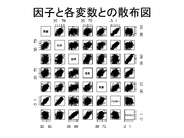
因子得点の算出 Factor Score for each sample • 因子負荷量と各個体のデータから算出 – 不確定性があり,複数の方法がある • バートレットの重み付き最小二乗法 • トムソンの回帰推定法 – factoanal(df, factors=n, scores="Bartlett", "regression", "none") ffive <- factanal(subjects, factors=2, scores="Bartlett") score <- data. frame(cbind(subjects, ffive$scores)) plot(score)
Rによる主成分分析 (分散共分散行列からはじめる) pca. gaku #固有値の平方根と固有ベクトルの表示 Standard deviations: [1] 13. 971074 9. 674429 6. 556847 5. 395683 5. 088521 Rotation: PC 1 PC 2 PC 3 PC 4 PC 5 国語 -0. 4545261 0. 6634739 -0. 47289752 0. 14516839 0. 32939713 社会 -0. 3667710 0. 2531514 0. 07138947 -0. 05134978 -0. 89087609 数学 -0. 3561308 -0. 2524045 0. 28362861 0. 85244739 0. 04848823 理科 -0. 5479742 -0. 6486996 -0. 45243098 -0. 27164715 0. 02066735 英語 -0. 4814356 0. 1058187 0. 69723203 -0. 41932160 0. 30831653
Rによる主成分分析 (分散共分散行列からはじめる) summary(pca. gaku) #固有値平方根,寄与率,累積寄与率 Importance of components: PC 1 Standard deviation 13. 971 Proportion of Variance 0. 505 Cumulative Proportion 0. 505 PC 2 9. 674 0. 242 0. 747 PC 3 6. 557 0. 111 0. 858 PC 4 5. 3957 0. 0753 0. 9331 PC 5 5. 089 0. 067 1. 000 cor(pca. gaku$x, subjects) #主成分負荷量:得点と原変数の相関 国語 社会 数学 理科 英語 PC 1 -0. 65302293 -0. 70318791 -0. 66851161 -0. 73343826 -0. 7778664 PC 2 0. 66006849 0. 33608746 -0. 32808926 -0. 60123277 0. 1183926 PC 3 -0. 31886138 0. 06423561 0. 24987036 -0. 28419803 0. 5287002 PC 4 0. 08054865 -0. 03802171 0. 61799311 -0. 14041879 -0. 2616560 PC 5 0. 17236584 -0. 62209333 0. 03315107 0. 01007511 0. 1814368
Rによる主成分分析 (相関係数行列からはじめる) pca. gaku 2 #固有値の平方根と固有ベクトルの表示 Standard deviations: [1] 1. 5992972 1. 0321853 0. 7111871 0. 6680076 0. 6517828 Rotation: PC 1 PC 2 PC 3 PC 4 PC 5 国語 -0. 4041725 0. 57887716 -0. 3519510 0. 3105217 0. 53033259 社会 -0. 4791143 0. 36327064 -0. 1060289 -0. 0743595 -0. 78848747 数学 -0. 4380351 -0. 48389701 0. 2494864 0. 7130299 -0. 05756589 理科 -0. 4064104 -0. 54428764 -0. 6058969 -0. 3977507 0. 11517295 英語 -0. 5000499 0. 05030239 0. 6599499 -0. 4810715 0. 28364804
Rによる主成分分析 (相関係数行列からはじめる) summary(pca. gaku 2) #固有値平方根,寄与率,累積寄与率 Importance of components: PC 1 Standard deviation 1. 599 Proportion of Variance 0. 512 Cumulative Proportion 0. 512 PC 2 1. 032 0. 213 0. 725 PC 3 0. 711 0. 101 0. 826 PC 4 0. 6680 0. 0892 0. 9150 PC 5 0. 652 0. 085 1. 000 cor(pca. gaku 2$x, subjects) #主成分負荷量:得点と原変数の相関 国語 社会 数学 理科 英語 PC 1 -0. 6463919 -0. 76624613 -0. 70054837 -0. 64997107 -0. 79972835 PC 2 0. 5975085 0. 37496261 -0. 49947137 -0. 56180569 0. 05192139 PC 3 -0. 2503030 -0. 07540635 0. 17743154 -0. 43090611 0. 46934784 PC 4 0. 2074308 -0. 04967271 0. 47630935 -0. 26570047 -0. 32135939 PC 5 0. 3456617 -0. 51392258 -0. 03752046 0. 07506775 0. 18487692