Paraguin Compiler Examples July 24 2012 copyright 2012
![Matrix Addition (complete) print_results(char *prompt, float a[N][N]) { int i, j; printf ("nn%sn", prompt); Matrix Addition (complete) print_results(char *prompt, float a[N][N]) { int i, j; printf ("nn%sn", prompt);](https://slidetodoc.com/presentation_image_h/044f3c181cf0d3b5540e968f198274da/image-10.jpg)

![; #pragma paraguin begin_parallel perm[0] = 0; min. Dist = -1. 0; if (n ; #pragma paraguin begin_parallel perm[0] = 0; min. Dist = -1. 0; if (n](https://slidetodoc.com/presentation_image_h/044f3c181cf0d3b5540e968f198274da/image-34.jpg)

![Sobel Edge Detection Algorithm /* 3 x 3 Sobel masks. */ GX[0][0] = -1; Sobel Edge Detection Algorithm /* 3 x 3 Sobel masks. */ GX[0][0] = -1;](https://slidetodoc.com/presentation_image_h/044f3c181cf0d3b5540e968f198274da/image-39.jpg)
- Slides: 42

Paraguin Compiler Examples July 24, 2012 © copyright 2012, Clayton S. Ferner, UNC Wilmington

Examples Matrix Addition (the complete program) Traveling Salesman Problem (TSP) Sobel Edge Detection July 24, 2012 © copyright 2012, Clayton S. Ferner, UNC Wilmington

Matrix Addition The complete program July 24, 2012 © copyright 2012, Clayton S. Ferner, UNC Wilmington

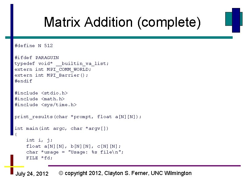
Matrix Addition (complete) #define N 512 #ifdef PARAGUIN typedef void* __builtin_va_list; extern int MPI_COMM_WORLD; extern int MPI_Barrier(); #endif #include <stdio. h> #include <math. h> #include <sys/time. h> print_results(char *prompt, float a[N][N]); int main(int argc, char *argv[]) { int i, j; float a[N][N], b[N][N], c[N][N]; char *usage = "Usage: %s filen"; FILE *fd; July 24, 2012 © copyright 2012, Clayton S. Ferner, UNC Wilmington

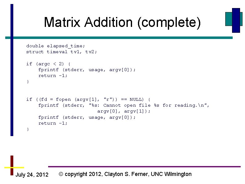
Matrix Addition (complete) double elapsed_time; struct timeval tv 1, tv 2; if (argc < 2) { fprintf (stderr, usage, argv[0]); return -1; } if ((fd = fopen (argv[1], "r")) == NULL) { fprintf (stderr, "%s: Cannot open file %s for reading. n", argv[0], argv[1]); fprintf (stderr, usage, argv[0]); return -1; } July 24, 2012 © copyright 2012, Clayton S. Ferner, UNC Wilmington

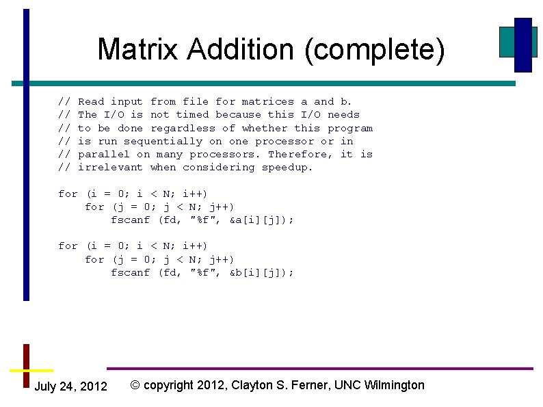
Matrix Addition (complete) // // // Read input from file for matrices a and b. The I/O is not timed because this I/O needs to be done regardless of whether this program is run sequentially on one processor or in parallel on many processors. Therefore, it is irrelevant when considering speedup. for (i = 0; i < N; i++) for (j = 0; j < N; j++) fscanf (fd, "%f", &a[i][j]); for (i = 0; i < N; i++) for (j = 0; j < N; j++) fscanf (fd, "%f", &b[i][j]); July 24, 2012 © copyright 2012, Clayton S. Ferner, UNC Wilmington

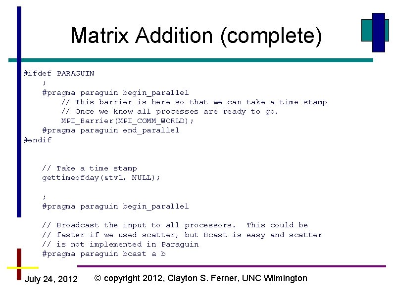
Matrix Addition (complete) #ifdef PARAGUIN ; #pragma paraguin begin_parallel // This barrier is here so that we can take a time stamp // Once we know all processes are ready to go. MPI_Barrier(MPI_COMM_WORLD); #pragma paraguin end_parallel #endif // Take a time stamp gettimeofday(&tv 1, NULL); ; #pragma paraguin begin_parallel // Broadcast the input to all processors. This could be // faster if we used scatter, but Bcast is easy and scatter // is not implemented in Paraguin #pragma paraguin bcast a b July 24, 2012 © copyright 2012, Clayton S. Ferner, UNC Wilmington

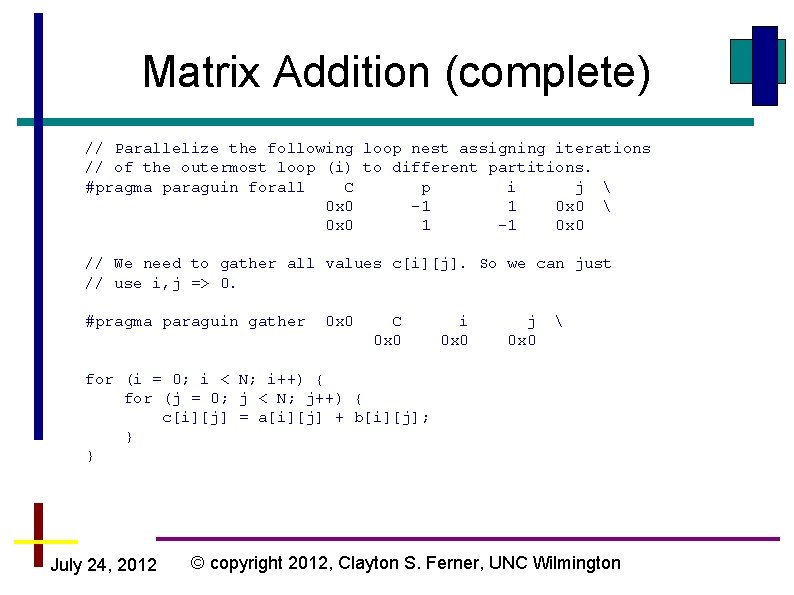
Matrix Addition (complete) // Parallelize the following loop nest assigning iterations // of the outermost loop (i) to different partitions. #pragma paraguin forall C p i j 0 x 0 -1 1 0 x 0 0 x 0 1 -1 0 x 0 // We need to gather all values c[i][j]. So we can just // use i, j => 0. #pragma paraguin gather 0 x 0 C 0 x 0 i 0 x 0 j 0 x 0 for (i = 0; i < N; i++) { for (j = 0; j < N; j++) { c[i][j] = a[i][j] + b[i][j]; } } July 24, 2012 © copyright 2012, Clayton S. Ferner, UNC Wilmington

Matrix Addition (complete) ; #pragma paraguin end_parallel // Take a time stamp. This won't happen until after the master // process has gathered all the input from the other processes. gettimeofday(&tv 2, NULL); elapsed_time = (tv 2. tv_sec - tv 1. tv_sec) + ((tv 2. tv_usec - tv 1. tv_usec) / 1000000. 0); printf ("elapsed_time=t%lf (seconds)n", elapsed_time); // print result print_results("C = ", c); } July 24, 2012 © copyright 2012, Clayton S. Ferner, UNC Wilmington
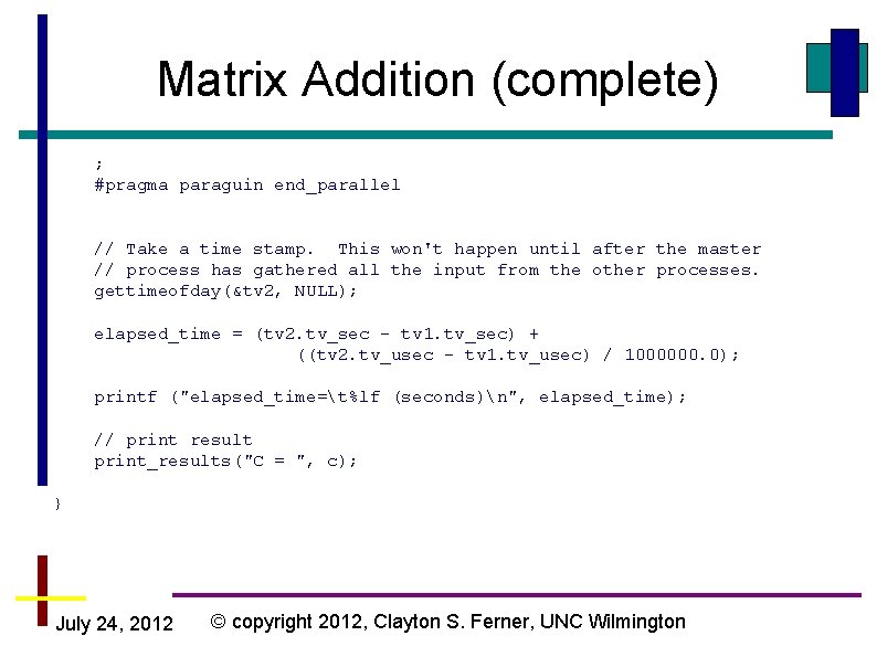
![Matrix Addition complete printresultschar prompt float aNN int i j printf nnsn prompt Matrix Addition (complete) print_results(char *prompt, float a[N][N]) { int i, j; printf ("nn%sn", prompt);](https://slidetodoc.com/presentation_image_h/044f3c181cf0d3b5540e968f198274da/image-10.jpg)
Matrix Addition (complete) print_results(char *prompt, float a[N][N]) { int i, j; printf ("nn%sn", prompt); for (i = 0; i < N; i++) { for (j = 0; j < N; j++) { printf(" %. 2 f", a[i][j]); } printf ("n"); } printf ("nn"); } July 24, 2012 © copyright 2012, Clayton S. Ferner, UNC Wilmington

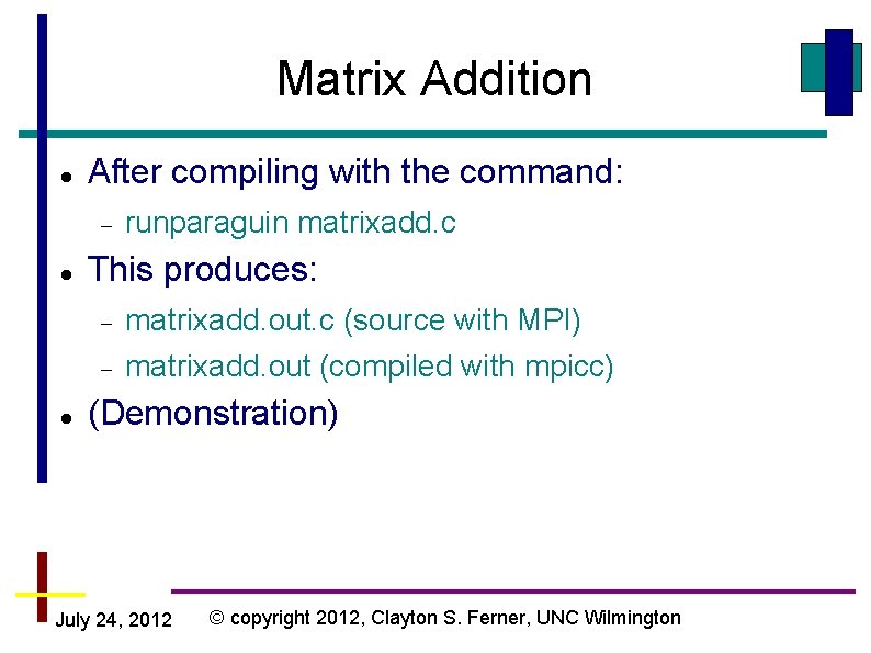
Matrix Addition After compiling with the command: This produces: runparaguin matrixadd. c matrixadd. out. c (source with MPI) matrixadd. out (compiled with mpicc) (Demonstration) July 24, 2012 © copyright 2012, Clayton S. Ferner, UNC Wilmington

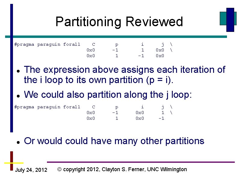
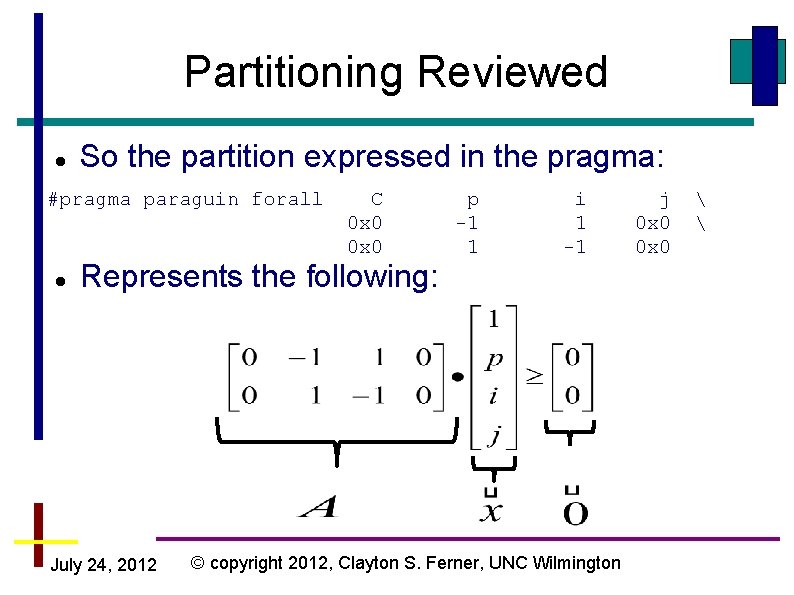
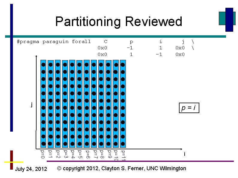
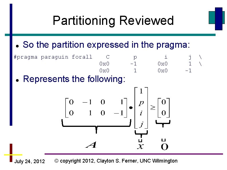
Partitioning Reviewed #pragma paraguin forall p -1 1 i 1 -1 j 0 x 0 The expression above assigns each iteration of the i loop to its own partition (p = i). We could also partition along the j loop: #pragma paraguin forall C 0 x 0 p -1 1 i 0 x 0 j 1 -1 Or would could have many other partitions July 24, 2012 © copyright 2012, Clayton S. Ferner, UNC Wilmington

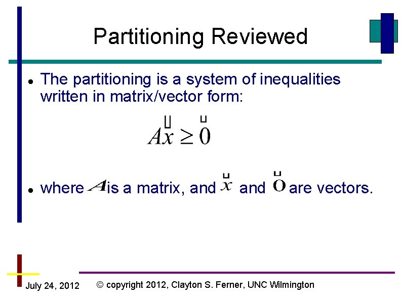
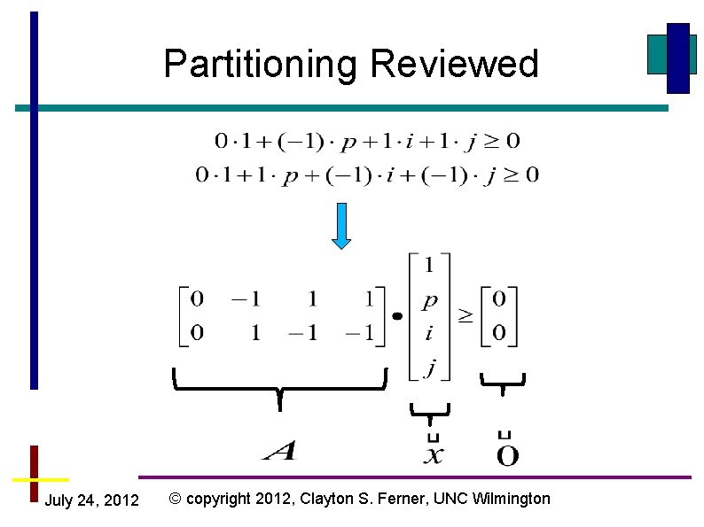
Partitioning Reviewed The partitioning is a system of inequalities written in matrix/vector form: where July 24, 2012 is a matrix, and are vectors. © copyright 2012, Clayton S. Ferner, UNC Wilmington

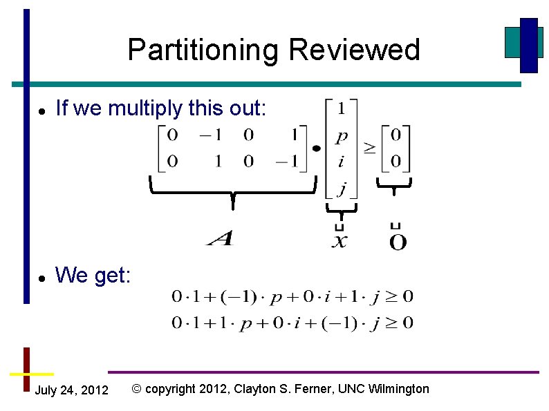
Partitioning Reviewed So the partition expressed in the pragma: #pragma paraguin forall C 0 x 0 Represents the following: July 24, 2012 p -1 1 i 1 -1 © copyright 2012, Clayton S. Ferner, UNC Wilmington j 0 x 0

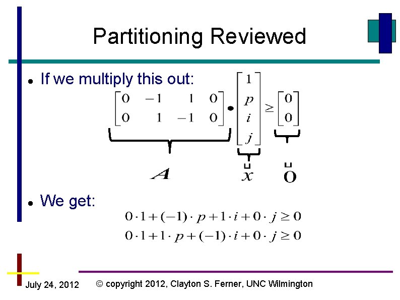
Partitioning Reviewed If we multiply this out: We get: July 24, 2012 © copyright 2012, Clayton S. Ferner, UNC Wilmington

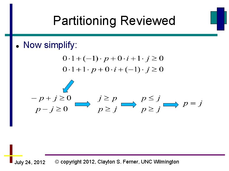
Partitioning Reviewed Now simplify: July 24, 2012 © copyright 2012, Clayton S. Ferner, UNC Wilmington

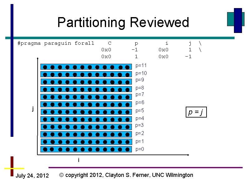
Partitioning Reviewed #pragma paraguin forall C 0 x 0 p -1 1 j i 1 -1 j 0 x 0 p=i p=11 p=10 p=9 p=8 p=7 p=6 p=5 p=4 p=3 p=2 p=1 p=0 July 24, 2012 i © copyright 2012, Clayton S. Ferner, UNC Wilmington

Partitioning Reviewed So the partition expressed in the pragma: #pragma paraguin forall C 0 x 0 Represents the following: July 24, 2012 p -1 1 i 0 x 0 © copyright 2012, Clayton S. Ferner, UNC Wilmington j 1 -1

Partitioning Reviewed If we multiply this out: We get: July 24, 2012 © copyright 2012, Clayton S. Ferner, UNC Wilmington

Partitioning Reviewed Now simplify: July 24, 2012 © copyright 2012, Clayton S. Ferner, UNC Wilmington

Partitioning Reviewed #pragma paraguin forall C 0 x 0 p -1 1 i 0 x 0 j 1 -1 p=11 p=10 p=9 p=8 p=7 p=6 j p=5 p=4 p=3 p=j p=2 p=1 p=0 i July 24, 2012 © copyright 2012, Clayton S. Ferner, UNC Wilmington

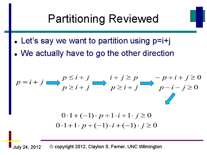
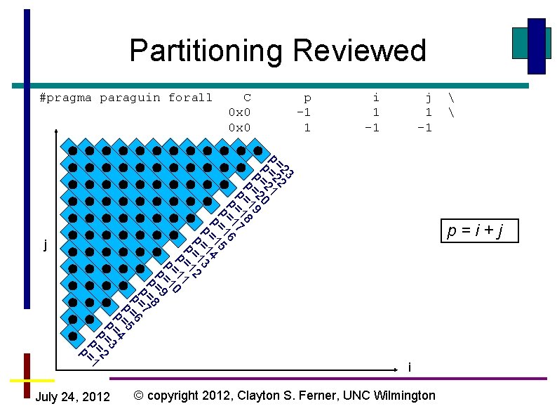
Partitioning Reviewed Let’s say we want to partition using p=i+j We actually have to go the other direction July 24, 2012 © copyright 2012, Clayton S. Ferner, UNC Wilmington

Partitioning Reviewed July 24, 2012 © copyright 2012, Clayton S. Ferner, UNC Wilmington

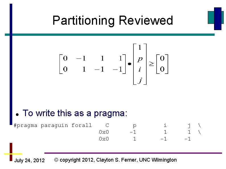
Partitioning Reviewed To write this as a pragma: #pragma paraguin forall July 24, 2012 C 0 x 0 p -1 1 i 1 -1 © copyright 2012, Clayton S. Ferner, UNC Wilmington j 1 -1

Partitioning Reviewed #pragma paraguin forall 23 2 p= =2 21 p 0 p= 2 9 p= 1 8 p= 1 7 p= =1 6 p 1 p= 15 4 p= 1 3 p= =1 2 p 1 p= 11 0 p= 1 p= =9 p 8 p= =7 p 6 p= =5 p 4 p= =3 p 2 p= =1 p j C 0 x 0 July 24, 2012 p -1 1 i 1 -1 j 1 -1 p=i+j i © copyright 2012, Clayton S. Ferner, UNC Wilmington

Traveling Salesman Problem (TSP) July 24, 2012 © copyright 2012, Clayton S. Ferner, UNC Wilmington

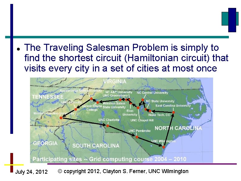
The Traveling Salesman Problem is simply to find the shortest circuit (Hamiltonian circuit) that visits every city in a set of cities at most once July 24, 2012 © copyright 2012, Clayton S. Ferner, UNC Wilmington

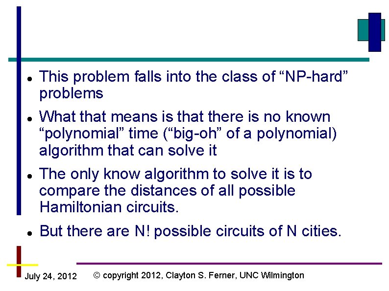
This problem falls into the class of “NP-hard” problems What that means is that there is no known “polynomial” time (“big-oh” of a polynomial) algorithm that can solve it The only know algorithm to solve it is to compare the distances of all possible Hamiltonian circuits. But there are N! possible circuits of N cities. July 24, 2012 © copyright 2012, Clayton S. Ferner, UNC Wilmington

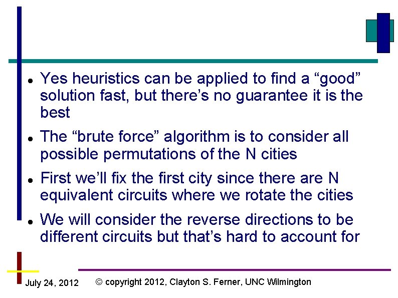
Yes heuristics can be applied to find a “good” solution fast, but there’s no guarantee it is the best The “brute force” algorithm is to consider all possible permutations of the N cities First we’ll fix the first city since there are N equivalent circuits where we rotate the cities We will consider the reverse directions to be different circuits but that’s hard to account for July 24, 2012 © copyright 2012, Clayton S. Ferner, UNC Wilmington

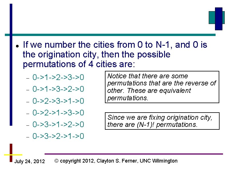
If we number the cities from 0 to N-1, and 0 is the origination city, then the possible permutations of 4 cities are: 0 ->1 ->2 ->3 ->0 0 ->1 ->3 ->2 ->0 0 ->2 ->3 ->1 ->0 0 ->2 ->1 ->3 ->0 0 ->3 ->1 ->2 ->0 0 ->3 ->2 ->1 ->0 July 24, 2012 Notice that there are some permutations that are the reverse of other. These are equivalent permutations. Since we are fixing origination city, there are (N-1)! permutations. © copyright 2012, Clayton S. Ferner, UNC Wilmington

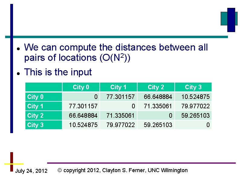
We can compute the distances between all pairs of locations (O(N 2)) This is the input City 0 City 1 City 2 City 3 City 0 0 77. 301157 66. 648884 10. 524875 City 1 77. 301157 0 71. 335061 79. 977022 City 2 66. 648884 71. 335061 0 59. 265103 City 3 10. 524875 79. 977022 59. 265103 0 July 24, 2012 © copyright 2012, Clayton S. Ferner, UNC Wilmington

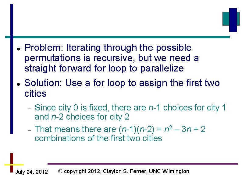
Problem: Iterating through the possible permutations is recursive, but we need a straight forward for loop to parallelize Solution: Use a for loop to assign the first two cities Since city 0 is fixed, there are n-1 choices for city 1 and n-2 choices for city 2 That means there are (n-1)(n-2) = n 2 – 3 n + 2 combinations of the first two cities July 24, 2012 © copyright 2012, Clayton S. Ferner, UNC Wilmington

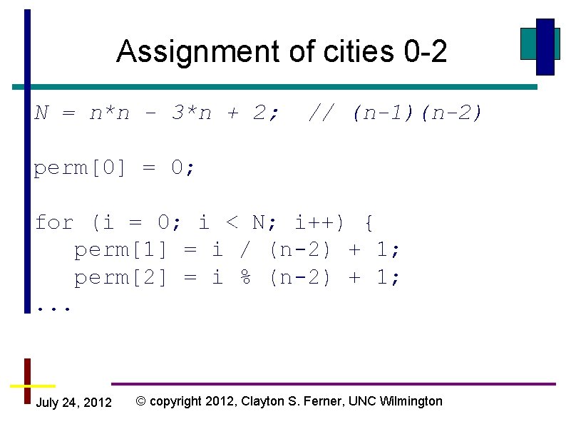
Assignment of cities 0 -2 N = n*n - 3*n + 2; // (n-1)(n-2) perm[0] = 0; for (i = 0; i < N; i++) { perm[1] = i / (n-2) + 1; perm[2] = i % (n-2) + 1; . . . July 24, 2012 © copyright 2012, Clayton S. Ferner, UNC Wilmington
![pragma paraguin beginparallel perm0 0 min Dist 1 0 if n ; #pragma paraguin begin_parallel perm[0] = 0; min. Dist = -1. 0; if (n](https://slidetodoc.com/presentation_image_h/044f3c181cf0d3b5540e968f198274da/image-34.jpg)
; #pragma paraguin begin_parallel perm[0] = 0; min. Dist = -1. 0; if (n == 2) { perm[1] = 1; // If n == 2, then N == 0, // and we are done. min. Perm[0] = perm[0]; min. Perm[1] = perm[1]; min. Dist = compute. Dist(D, n, perm); } ; #pragma paraguin bcast n #pragma paraguin bcast N #pragma paraguin bcast D July 24, 2012 © copyright 2012, Clayton S. Ferner, UNC Wilmington

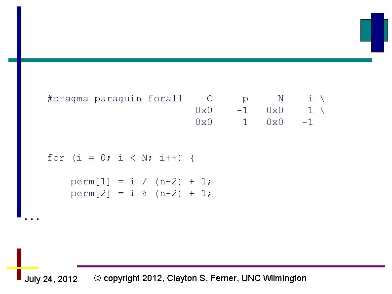
#pragma paraguin forall C 0 x 0 p -1 1 N 0 x 0 i 1 -1 for (i = 0; i < N; i++) { perm[1] = i / (n-2) + 1; perm[2] = i % (n-2) + 1; . . . July 24, 2012 © copyright 2012, Clayton S. Ferner, UNC Wilmington

Sobel Edge Detection July 24, 2012 © copyright 2012, Clayton S. Ferner, UNC Wilmington

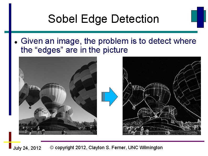
Sobel Edge Detection Given an image, the problem is to detect where the “edges” are in the picture July 24, 2012 © copyright 2012, Clayton S. Ferner, UNC Wilmington

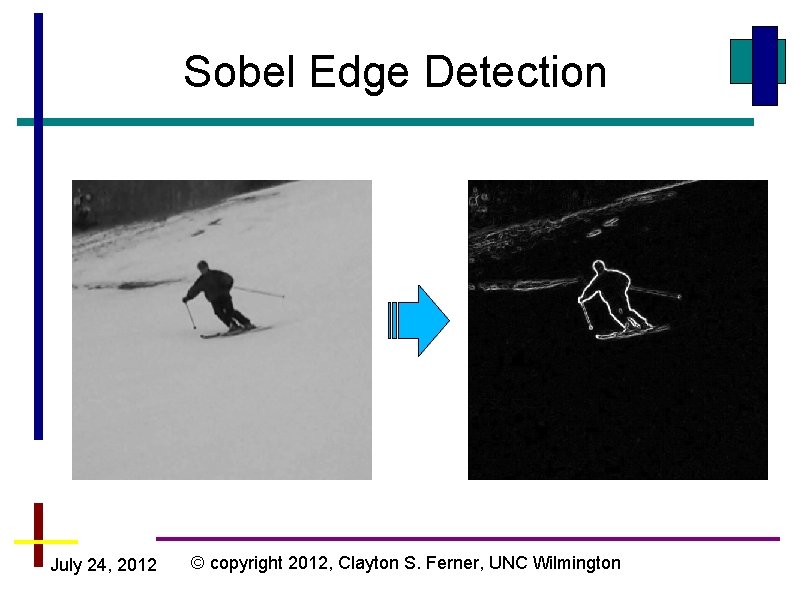
Sobel Edge Detection July 24, 2012 © copyright 2012, Clayton S. Ferner, UNC Wilmington
![Sobel Edge Detection Algorithm 3 x 3 Sobel masks GX00 1 Sobel Edge Detection Algorithm /* 3 x 3 Sobel masks. */ GX[0][0] = -1;](https://slidetodoc.com/presentation_image_h/044f3c181cf0d3b5540e968f198274da/image-39.jpg)
Sobel Edge Detection Algorithm /* 3 x 3 Sobel masks. */ GX[0][0] = -1; GX[0][1] = 0; GX[0][2] = 1; GX[1][0] = -2; GX[1][1] = 0; GX[1][2] = 2; GX[2][0] = -1; GX[2][1] = 0; GX[2][2] = 1; GY[0][0] = 1; GY[0][1] = 2; GY[0][2] = 1; GY[1][0] = 0; GY[1][1] = 0; GY[1][2] = 0; GY[2][0] = -1; GY[2][1] = -2; GY[2][2] = -1; for(x=0; x < N; ++x){ for(y=0; y < N; ++y){ sumx = 0; sumy = 0; // handle image boundaries if(x==0 || x==(h-1) || y==0 || y==(w-1)) sum = 0; else{ July 24, 2012 Pragmas go here © copyright 2012, Clayton S. Ferner, UNC Wilmington

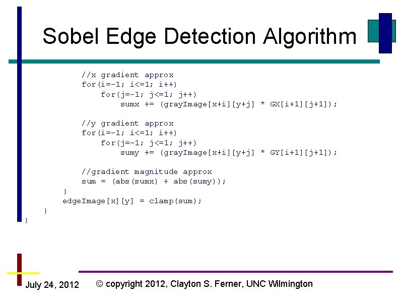
Sobel Edge Detection Algorithm //x gradient approx for(i=-1; i<=1; i++) for(j=-1; j<=1; j++) sumx += (gray. Image[x+i][y+j] * GX[i+1][j+1]); //y gradient approx for(i=-1; i<=1; i++) for(j=-1; j<=1; j++) sumy += (gray. Image[x+i][y+j] * GY[i+1][j+1]); //gradient magnitude approx sum = (abs(sumx) + abs(sumy)); } edge. Image[x][y] = clamp(sum); } } July 24, 2012 © copyright 2012, Clayton S. Ferner, UNC Wilmington

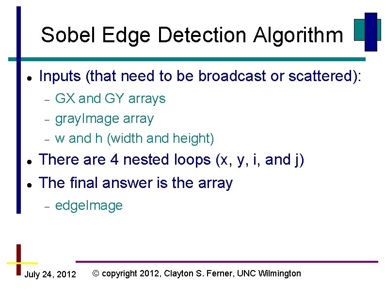
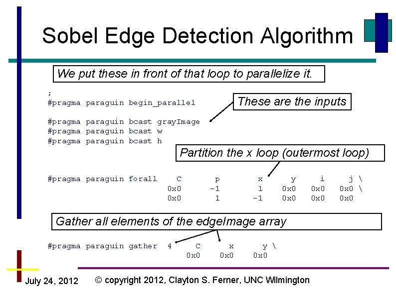
Sobel Edge Detection Algorithm Inputs (that need to be broadcast or scattered): GX and GY arrays gray. Image array w and h (width and height) There are 4 nested loops (x, y, i, and j) The final answer is the array edge. Image July 24, 2012 © copyright 2012, Clayton S. Ferner, UNC Wilmington

Sobel Edge Detection Algorithm We put these in front of that loop to parallelize it. ; #pragma paraguin begin_parallel These are the inputs #pragma paraguin bcast gray. Image #pragma paraguin bcast w #pragma paraguin bcast h Partition the x loop (outermost loop) #pragma paraguin forall C 0 x 0 p -1 1 x 1 -1 y 0 x 0 Gather all elements of the edge. Image array #pragma paraguin gather July 24, 2012 4 C 0 x 0 x 0 x 0 y 0 x 0 © copyright 2012, Clayton S. Ferner, UNC Wilmington i 0 x 0 j 0 x 0