Pairwise Structural Comparison using DALILite Software of DALI

Pair-wise Structural Comparison using DALILite Software of DALI Rajalekshmy Usha

Overview n n n n History Protein Structure Comparison Algorithm Input and Output Interface Demo on the software Analysis of the Result References

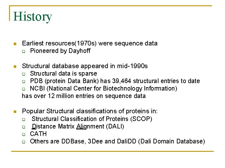
History n Earliest resources(1970 s) were sequence data q Pioneered by Dayhoff n Structural database appeared in mid-1990 s q Structural data is sparse q PDB (protein Data Bank) has 39, 464 structural entries to date q NCBI (National Center for Biotechnology Information) has over 12 million entries on sequence data n Popular Structural classifications of proteins in: q Structural Classification of Proteins (SCOP) q Distance Matrix Alignment (DALI) q CATH q Others are DDBase, 3 Dee and Dali. DD (Dali Domain Database)

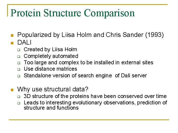
Protein Structure Comparison n n Popularized by Liisa Holm and Chris Sander (1993) DALI q q q n Created by Liisa Holm Completely automated Too large and complex to be installed in external sites Use distance matrices Standalone version of search engine of Dali server Why use structural data? q q 3 D structure of the proteins have been conserved over time Leads to interesting evolutionary observations, prediction of structure and functions

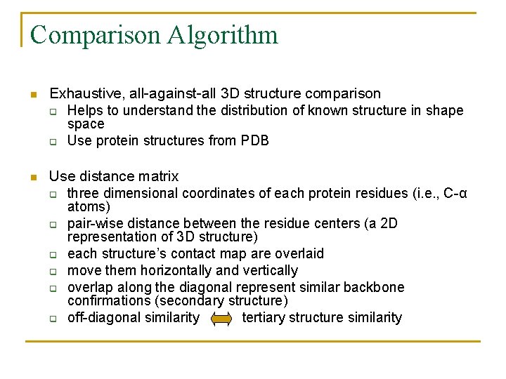
Comparison Algorithm n Exhaustive, all-against-all 3 D structure comparison q Helps to understand the distribution of known structure in shape space q Use protein structures from PDB n Use distance matrix q three dimensional coordinates of each protein residues (i. e. , C-α atoms) q pair-wise distance between the residue centers (a 2 D representation of 3 D structure) q each structure’s contact map are overlaid q move them horizontally and vertically q overlap along the diagonal represent similar backbone confirmations (secondary structure) q off-diagonal similarity tertiary structure similarity

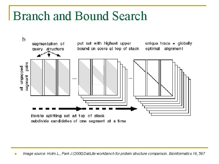
Underlying Algorithms n Branch and Bound Search to find the optimal alignment q Uses distance matrices n n q n Collapsed into regions of overlap (sub-matrices) of fixed size The sub-matrices are stitched together if there is an overlap with the neighboring fragments Uses similarity score Monte Carlo Optimization Algorithm q To optimize the alignment

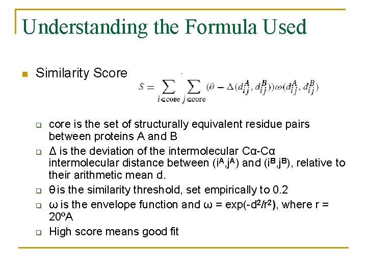
Understanding the Formula Used n Similarity Score q q q core is the set of structurally equivalent residue pairs between proteins A and B Δ is the deviation of the intermolecular Cα-Cα intermolecular distance between (i. A, j. A) and (i. B, j. B), relative to their arithmetic mean d. θ is the similarity threshold, set empirically to 0. 2 ω is the envelope function and ω = exp(-d 2/r 2), where r = 20ºA High score means good fit

Branch and Bound Search n Consider only nongapped segment pairs q q This reduces the complexity of structure alignment Natural segmentation uses the secondary structures of the query structure n n Diagonal lines represent the nongapped segment pairings q n n E. g. α helices and β strands Pairing between segments of query structure (horizontal) and the proteins being aligned to it (vertical). Do an alignment score (similarity score) within the segments and between the segments Split the search space into smaller subset of candidate pairings (matrices) Chose the upper bound on the sum-of-pairs score Subset with the highest bound contains the optimal alignment

Branch and Bound Search n Image source: Holm L. , Park J (2000)Dali. Lite workbench for protein structure comparison. Bioinformatics 16, 567

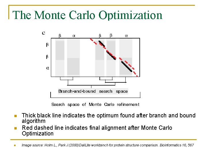
Monte Carlo Optimization Algorithm n A basic move is made q The move is random n q n Probability of accepting a move is p = e beta*(s’-s), where S’ = new score, S= old score and beta is a parameter Involves addition or deletion of residue equivalence assignment Two basic modes of operation q Expansion mode n n q Alignment is incremented by using overlapping contact patterns Extend the alignment by including all pairs of matching contact patterns with the same residue pairs (i. A , i. B) Adding new fragment requires tentative removal of inconsistent previous equivalent assignment The removal is permanent Trimming mode n n Removal of fragment that give a net negative contribution to the similarity score Done after the 1 st and every 5 subsequent expansion cycles

The Monte Carlo Optimization n Thick black line indicates the optimum found after branch and bound algorithm Red dashed line indicates final alignment after Monte Carlo Optimization Image source: Holm L. , Park J (2000)Dali. Lite workbench for protein structure comparison. Bioinformatics 16, 567

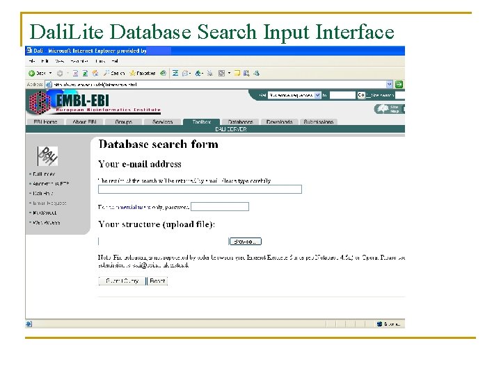
Dali. Lite Database Search Input Interface

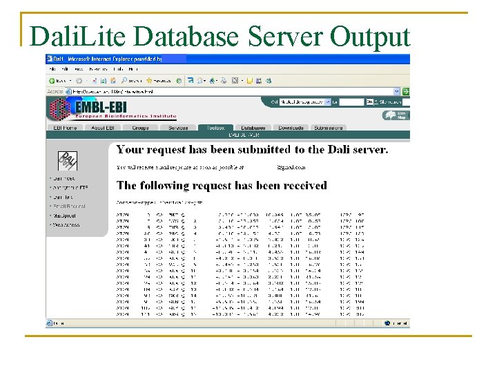
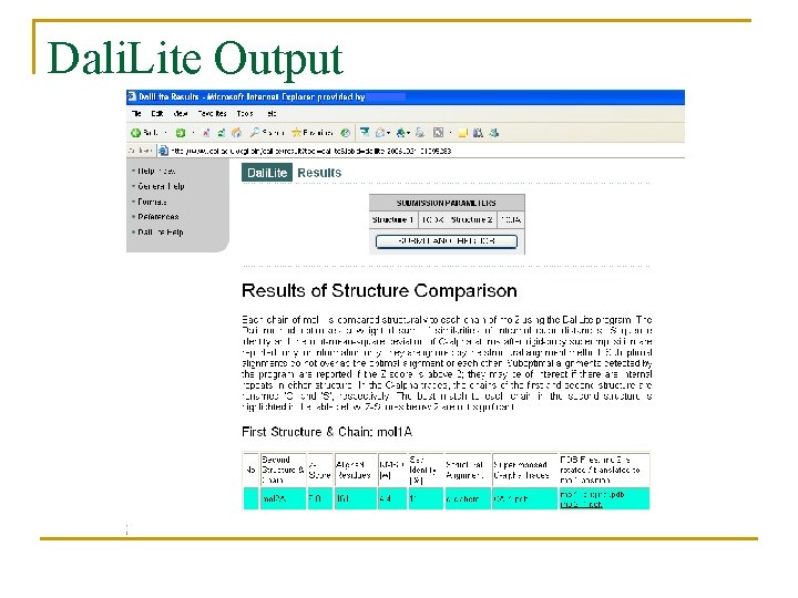
Dali. Lite Database Server Output

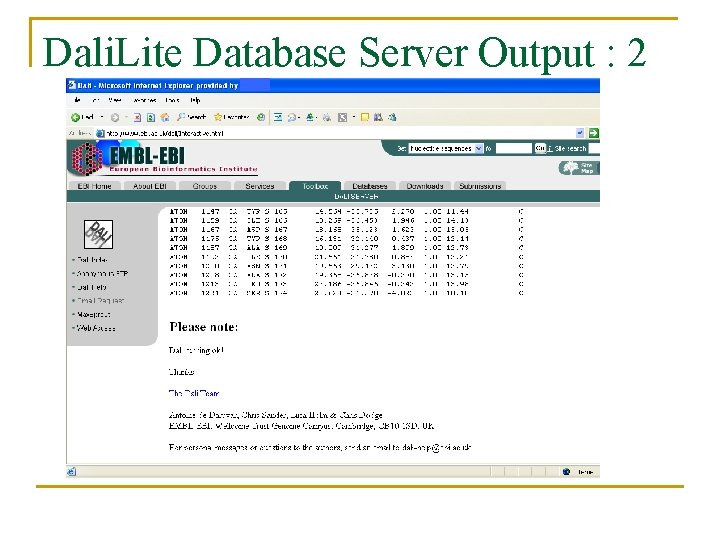
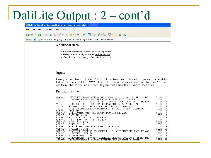
Dali. Lite Database Server Output : 2

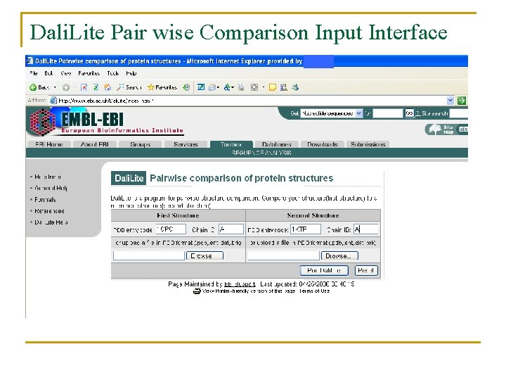
Dali. Lite Pair wise Comparison Input Interface

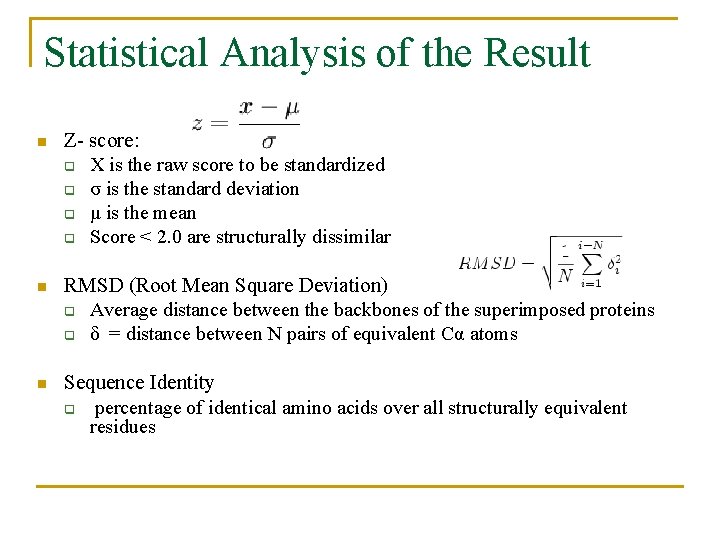
Statistical Analysis of the Result n Z- score: q X is the raw score to be standardized q σ is the standard deviation q μ is the mean q Score < 2. 0 are structurally dissimilar n RMSD (Root Mean Square Deviation) q Average distance between the backbones of the superimposed proteins q δ = distance between N pairs of equivalent Cα atoms n Sequence Identity q percentage of identical amino acids over all structurally equivalent residues

Dali. Lite Output

Dali. Lite Output : 2 – cont’d

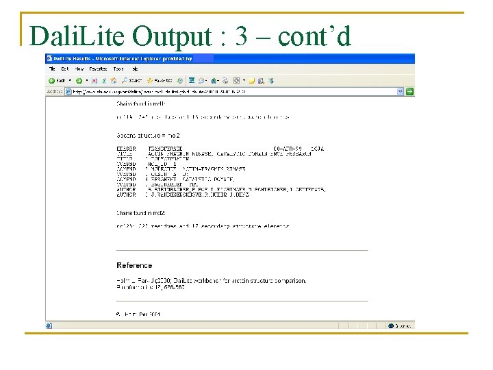
Dali. Lite Output : 3 – cont’d

Demo on Using Dali. Lite n http: //www. ebi. ac. uk/dali/index. html

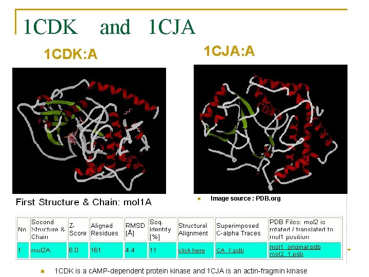
1 CDK and 1 CJA: A 1 CDK: A n n Image source : PDB. org 1 CDK is a c. AMP-dependent protein kinase and 1 CJA is an actin-fragmin kinase

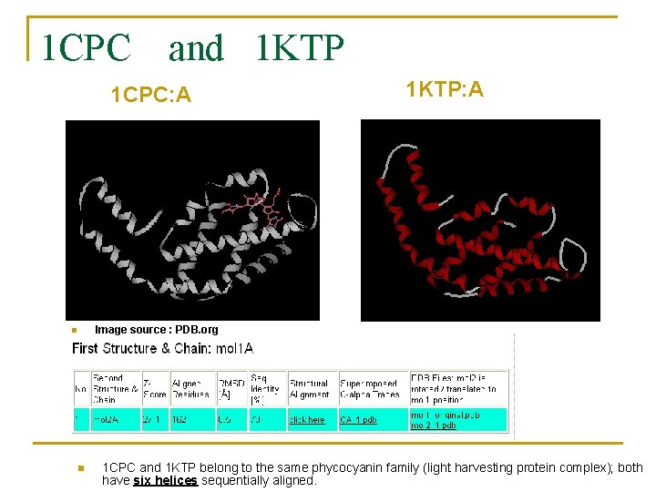
1 CPC and 1 KTP 1 CPC: A 1 KTP: A Image source : PDB. org n n 1 CPC and 1 KTP belong to the same phycocyanin family (light harvesting protein complex); both have six helices sequentially aligned.

References n n n Holm L. , Sander C(1993 a) Protein Structure Comparison by Alignment of Distance Matrices. Journal of Molecular Biol. 233(1): 123 -138 Holm L. , Park J(2000) Dali. Lite workbench for protein structure comparison. Bioinformatics 16, 566 -567 Holm L. , Sander C(1996) Mapping the protein universe. Science 273: 595 -602 Bourne P. E. , Weissig H. Structural Bioinformatics. Wiley-Liss, Hoboken, New Jersey http: //wikipedia. org