Microsoft Excel 2010 Chapter 3 WhatIf Analysis Charting

Microsoft Excel 2010 Chapter 3 What-If Analysis, Charting, and Working with Large Worksheets

Objectives Rotate text in a cell Create a series of month names Copy, paste, insert, and delete cells Format numbers using format symbols Freeze and unfreeze rows and columns Show and format the system date Use absolute and mixed cell references in a formula • Use the IF function to perform a logical test • • What-If Analysis, Charting, and Working with Large Worksheets 2

Objectives • • Create Sparkline charts Use the Format Painter button to format cells Create a 3 -D Pie chart on a separate chart sheet Rearrange worksheet tabs Change the worksheet view Answer what-if questions Goal seek to answer what-if questions What-If Analysis, Charting, and Working with Large Worksheets 3

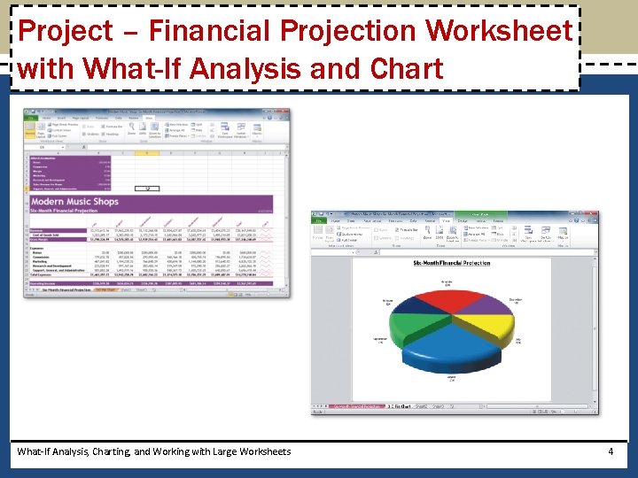
Project – Financial Projection Worksheet with What-If Analysis and Chart What-If Analysis, Charting, and Working with Large Worksheets 4

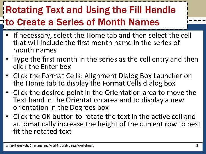
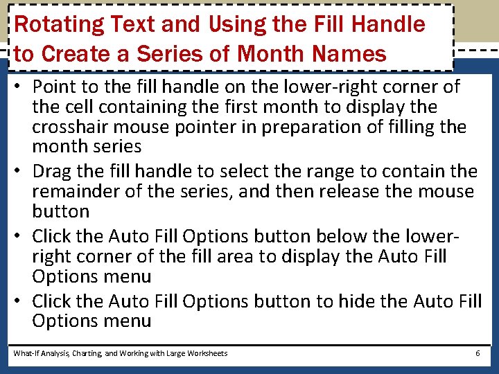
Rotating Text and Using the Fill Handle to Create a Series of Month Names • If necessary, select the Home tab and then select the cell that will include the first month name in the series of month names • Type the first month in the series as the cell entry and then click the Enter box • Click the Format Cells: Alignment Dialog Box Launcher on the Home tab to display the Format Cells dialog box • Click the desired point in the Orientation area to move the Text hand in the Orientation area and to display a new orientation in the Degrees box • Click the OK button to rotate the text in the active cell and automatically increase the height of the current row to best fit the rotated text What-If Analysis, Charting, and Working with Large Worksheets 5

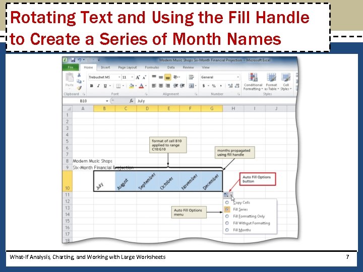
Rotating Text and Using the Fill Handle to Create a Series of Month Names • Point to the fill handle on the lower-right corner of the cell containing the first month to display the crosshair mouse pointer in preparation of filling the month series • Drag the fill handle to select the range to contain the remainder of the series, and then release the mouse button • Click the Auto Fill Options button below the lowerright corner of the fill area to display the Auto Fill Options menu • Click the Auto Fill Options button to hide the Auto Fill Options menu What-If Analysis, Charting, and Working with Large Worksheets 6

Rotating Text and Using the Fill Handle to Create a Series of Month Names What-If Analysis, Charting, and Working with Large Worksheets 7

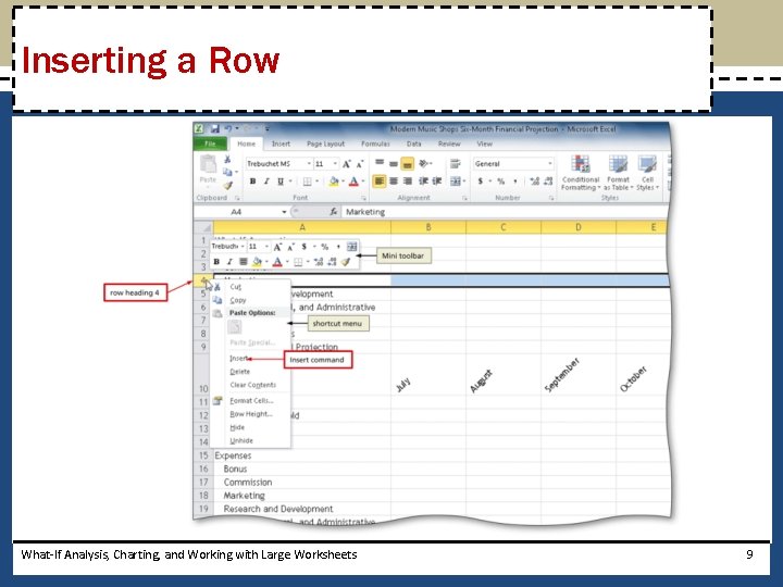
Inserting a Row • Right-click the row heading below where you want to insert a row to display the shortcut menu and the Mini toolbar • Click Insert on the shortcut menu to insert a new row in the worksheet by shifting the selected row and all rows below it down one row What-If Analysis, Charting, and Working with Large Worksheets 8

Inserting a Row What-If Analysis, Charting, and Working with Large Worksheets 9

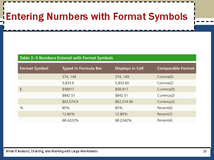
Entering Numbers with Format Symbols What-If Analysis, Charting, and Working with Large Worksheets 10

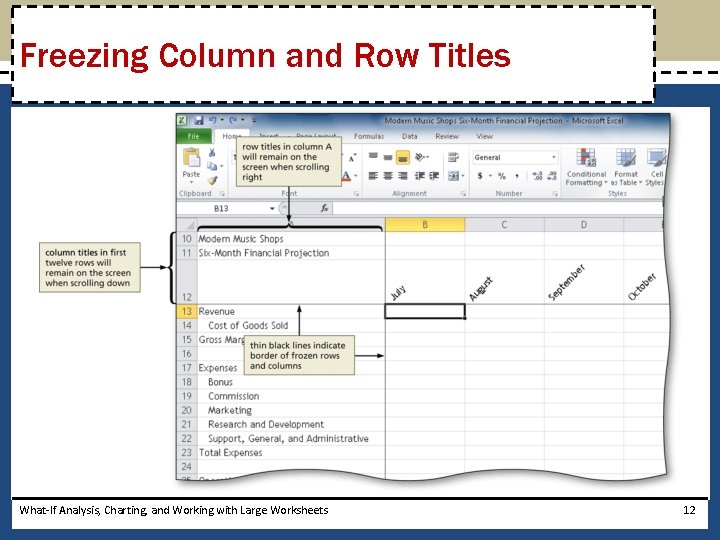
Freezing Column and Row Titles • Select the cell on which to freeze panes • Display the View tab and then click the Freeze Panes button to display the Freeze Panes gallery • Click Freeze Panes in the Freeze Panes gallery to freeze rows and columns to the left and above the selected cell What-If Analysis, Charting, and Working with Large Worksheets 11

Freezing Column and Row Titles What-If Analysis, Charting, and Working with Large Worksheets 12

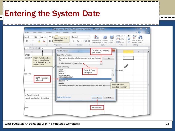
Entering the System Date • Select the cell in which you want to insert the date, and then click the Insert Function box in the formula bar to display the Insert Function dialog box • Click the ‘Or select a category’ box arrow and then select Date & Time in the list to populate the ‘Select a function’ list with date and time functions • Scroll down in the ‘Select a function list’ and then click NOW to select the function • Click the OK button to close the Insert Function dialog box • Click the OK button to display the system date and time in the selected cell What-If Analysis, Charting, and Working with Large Worksheets 13

Entering the System Date What-If Analysis, Charting, and Working with Large Worksheets 14

Absolute versus Relative Addressing What-If Analysis, Charting, and Working with Large Worksheets 15

Absolute versus Relative Addressing What-If Analysis, Charting, and Working with Large Worksheets 16

Entering an IF Function • Click the cell to contain the formula, and then click the Insert Function box in the formula bar to display the Insert Function dialog box • Click the ‘Or select a category’ box arrow and then select Logical in the list to populate the ‘Select a function’ list with logic functions • Click IF in the ‘Select a function list’ to select the required function • Click the OK button to display the Function Arguments dialog box What-If Analysis, Charting, and Working with Large Worksheets 17

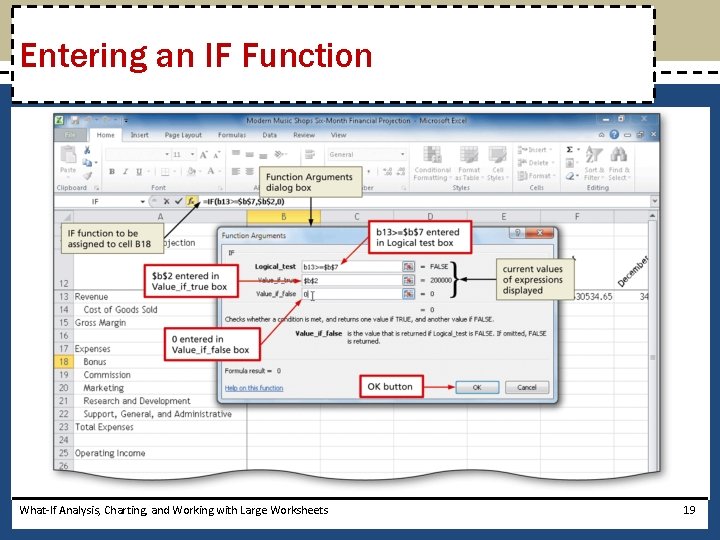
Entering an IF Function • Enter the logical test in the Logical text box to enter a logical test for the IF function • Type the result of the IF function if the logical test is true in the Value_if_true box • Type the result of the IF function if the logical test is false in the Value_if_false box • Click the OK button to insert the IF function in the selected cell What-If Analysis, Charting, and Working with Large Worksheets 18

Entering an IF Function What-If Analysis, Charting, and Working with Large Worksheets 19

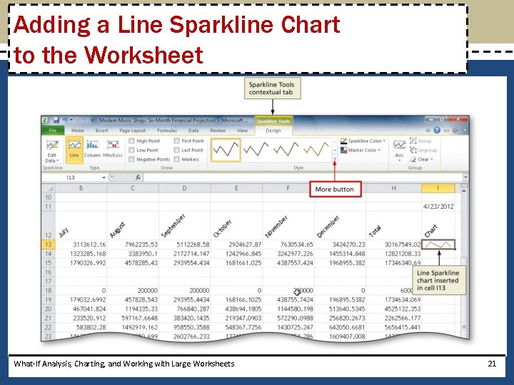
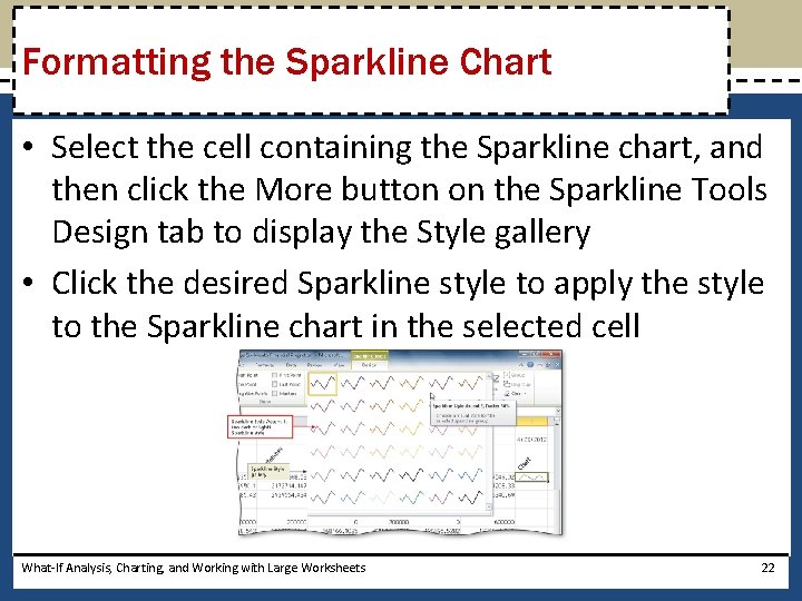
Adding a Line Sparkline Chart to the Worksheet • Select the cell in which you want to insert a Sparkline chart • Display the Insert tab and then click Line to display the Create Sparklines dialog box • Drag through the range of cells of which you want to chart, and then release the mouse button to insert the selected range in the Data Range text box • Click the OK button to insert a Line Sparkline chart in the selected cell and display the Sparkline Tools contextual tab What-If Analysis, Charting, and Working with Large Worksheets 20

Adding a Line Sparkline Chart to the Worksheet What-If Analysis, Charting, and Working with Large Worksheets 21

Formatting the Sparkline Chart • Select the cell containing the Sparkline chart, and then click the More button on the Sparkline Tools Design tab to display the Style gallery • Click the desired Sparkline style to apply the style to the Sparkline chart in the selected cell What-If Analysis, Charting, and Working with Large Worksheets 22

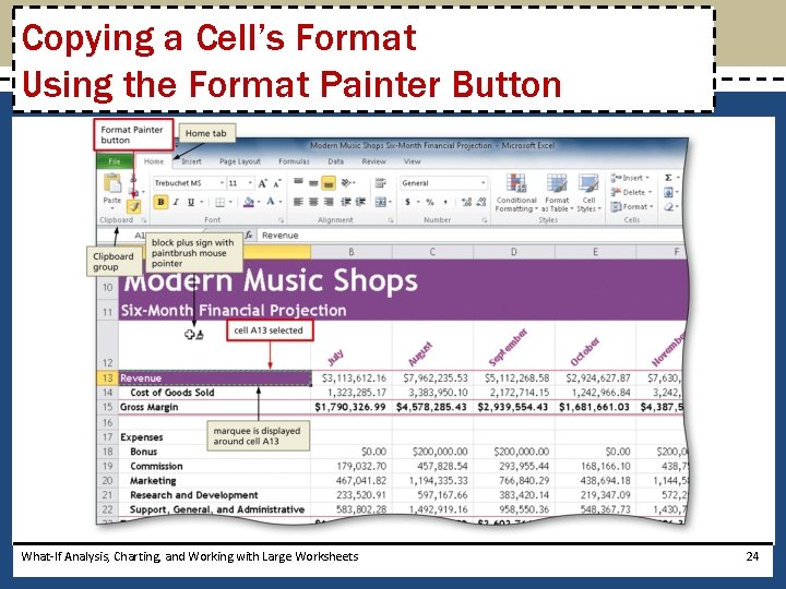
Copying a Cell’s Format Using the Format Painter Button • Select the source cell for the format to paint • Double-click the Format Painter button on the Home tab • Click the cell(s) to receive the format to assign the format of the source cell to the destination cell(s) • Press the ESC key to stop the format painter What-If Analysis, Charting, and Working with Large Worksheets 23

Copying a Cell’s Format Using the Format Painter Button What-If Analysis, Charting, and Working with Large Worksheets 24

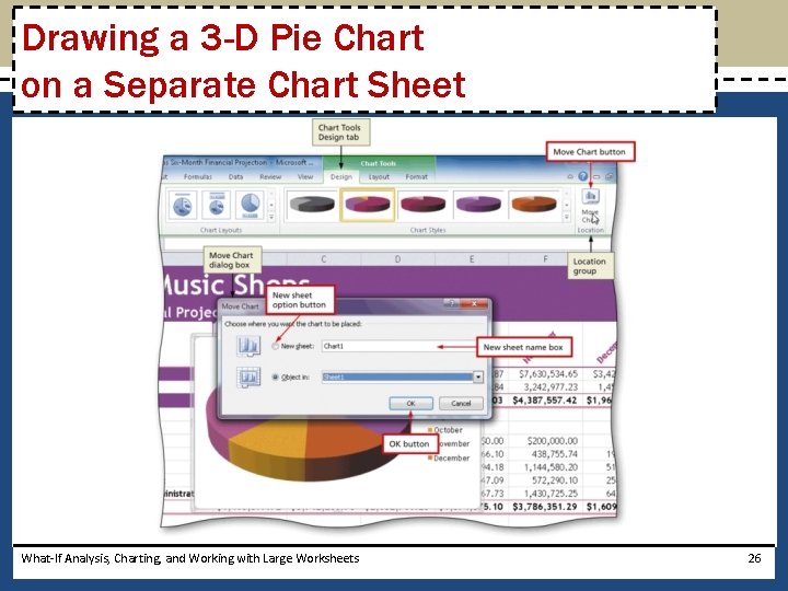
Drawing a 3 -D Pie Chart on a Separate Chart Sheet • Select the range of cells to include in the chart • Click the Pie button on the Insert tab to display the Pie gallery • Click the desired chart type in the Pie gallery • Click the Move Chart button on the Chart Tools Design tab to display the Move Chart dialog box • Click New sheet, and then type the name of the sheet tab for the chart sheet • Click the OK button to move the chart to a new chart sheet What-If Analysis, Charting, and Working with Large Worksheets 25

Drawing a 3 -D Pie Chart on a Separate Chart Sheet What-If Analysis, Charting, and Working with Large Worksheets 26

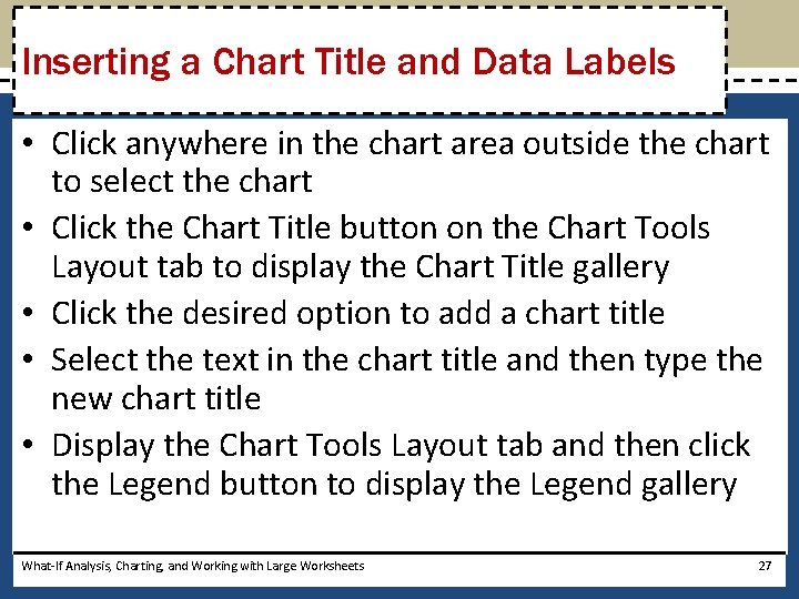
Inserting a Chart Title and Data Labels • Click anywhere in the chart area outside the chart to select the chart • Click the Chart Title button on the Chart Tools Layout tab to display the Chart Title gallery • Click the desired option to add a chart title • Select the text in the chart title and then type the new chart title • Display the Chart Tools Layout tab and then click the Legend button to display the Legend gallery What-If Analysis, Charting, and Working with Large Worksheets 27

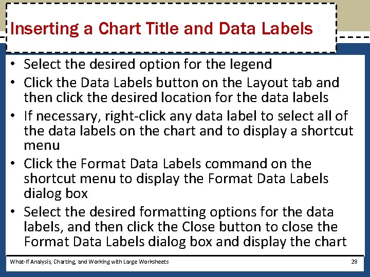
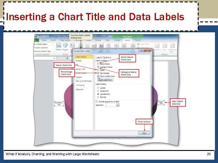
Inserting a Chart Title and Data Labels • Select the desired option for the legend • Click the Data Labels button on the Layout tab and then click the desired location for the data labels • If necessary, right-click any data label to select all of the data labels on the chart and to display a shortcut menu • Click the Format Data Labels command on the shortcut menu to display the Format Data Labels dialog box • Select the desired formatting options for the data labels, and then click the Close button to close the Format Data Labels dialog box and display the chart What-If Analysis, Charting, and Working with Large Worksheets 28

Inserting a Chart Title and Data Labels What-If Analysis, Charting, and Working with Large Worksheets 29

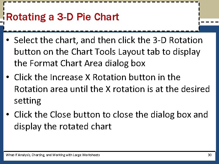
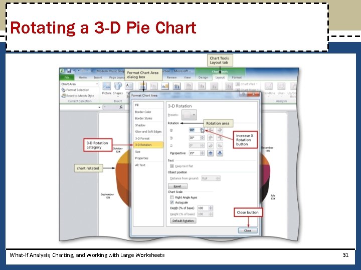
Rotating a 3 -D Pie Chart • Select the chart, and then click the 3 -D Rotation button on the Chart Tools Layout tab to display the Format Chart Area dialog box • Click the Increase X Rotation button in the Rotation area until the X rotation is at the desired setting • Click the Close button to close the dialog box and display the rotated chart What-If Analysis, Charting, and Working with Large Worksheets 30

Rotating a 3 -D Pie Chart What-If Analysis, Charting, and Working with Large Worksheets 31

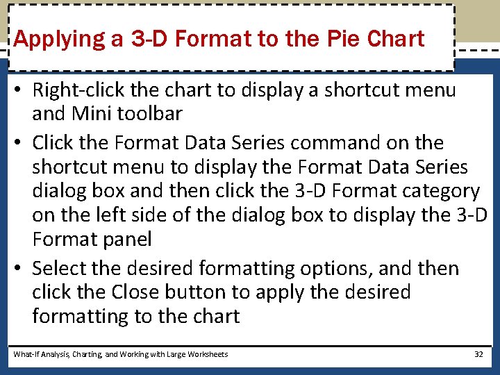
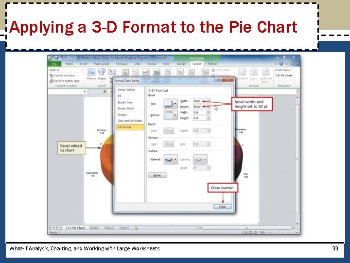
Applying a 3 -D Format to the Pie Chart • Right-click the chart to display a shortcut menu and Mini toolbar • Click the Format Data Series command on the shortcut menu to display the Format Data Series dialog box and then click the 3 -D Format category on the left side of the dialog box to display the 3 -D Format panel • Select the desired formatting options, and then click the Close button to apply the desired formatting to the chart What-If Analysis, Charting, and Working with Large Worksheets 32

Applying a 3 -D Format to the Pie Chart What-If Analysis, Charting, and Working with Large Worksheets 33

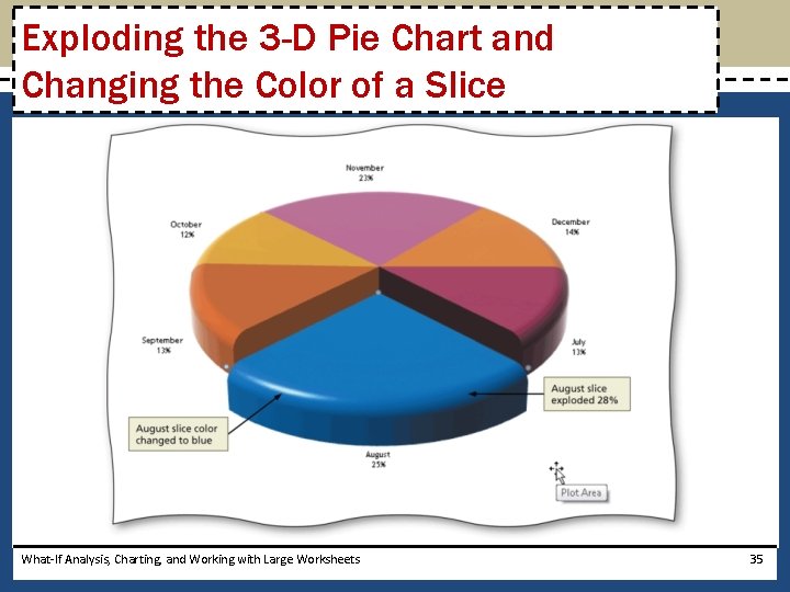
Exploding the 3 -D Pie Chart and Changing the Color of a Slice • Click the slice to explode twice (do not double-click), and then right-click the slice to display a shortcut menu and Mini toolbar • Click Format Data Point on the shortcut menu to display the Format Data Point dialog box • Drag the Point Explosion slider to the desired location to set how far the slice in the 3 -D Pie Chart should be offset from the rest of the chart • Click the Fill category on the left side of the dialog box to display the Fill panel • Click the desired fill type, and then click the Color button to display the Color gallery • Click the desired color in the color gallery and then click the Close button to change the color of the selected slice and close the dialog box What-If Analysis, Charting, and Working with Large Worksheets 34

Exploding the 3 -D Pie Chart and Changing the Color of a Slice What-If Analysis, Charting, and Working with Large Worksheets 35

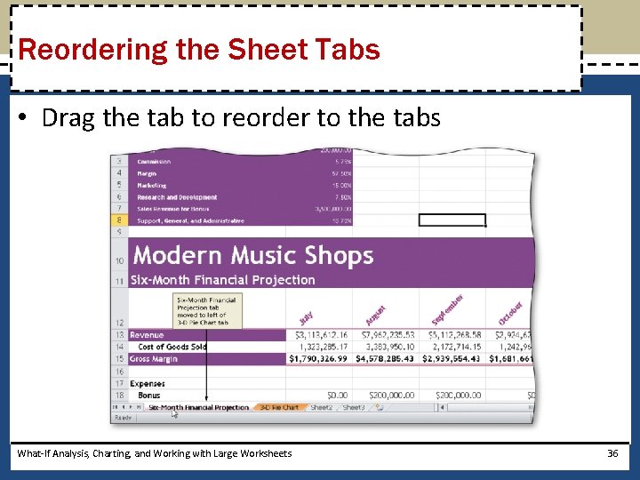
Reordering the Sheet Tabs • Drag the tab to reorder to the tabs What-If Analysis, Charting, and Working with Large Worksheets 36

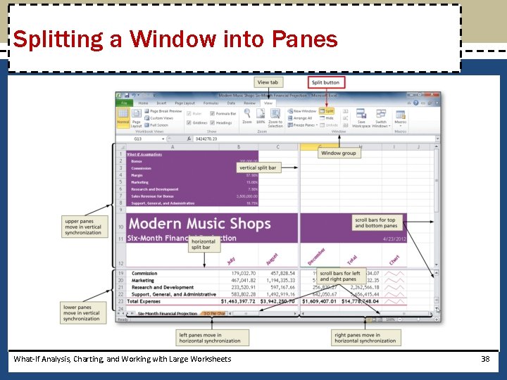
Splitting a Window into Panes • Click the cell at the intersection of the four proposed panes to select the cell at which to split the window • Click the Split button on the View tab to divide the window into four panes What-If Analysis, Charting, and Working with Large Worksheets 37

Splitting a Window into Panes What-If Analysis, Charting, and Working with Large Worksheets 38

What-If Analysis • The automatic recalculation feature of Excel is a powerful tool that can be used to analyze worksheet data • Using Excel to scrutinize the impact of changing values in cells that are referenced by a formula in another cell is called what-if analysis or sensitivity analysis What-If Analysis, Charting, and Working with Large Worksheets 39

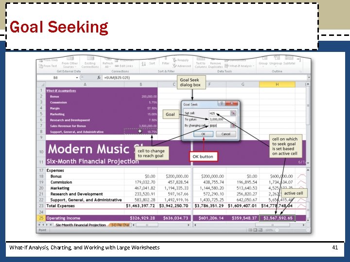
Goal Seeking • If you know the result you want a formula to produce, you can use goal seeking to determine the value of a cell on which the formula depends – Goal Seek command on the Data tab • Goal seeking assumes you can change the value of only one cell referenced directly or indirectly to reach a specific goal for a value in another cell What-If Analysis, Charting, and Working with Large Worksheets 40

Goal Seeking What-If Analysis, Charting, and Working with Large Worksheets 41